UPDATE: In response to Jarrett’s query I laid out a separate use case in which you may want to query by higher taxonomic rankings than species. See below. In addition, added examples of querying by location in reply to comments by seminym.
We have been working on an R package to get GBIF data from R, with the stable version available through CRAN, and the development version available on GitHub at https://github.com/rgbif
We had a Google Summer of code stuent work on the package this summer - you can see his work on the package over at his GitHub page here. We have added some new functionality since his work, and would like to show it off.
Install
# install_github('rgbif', 'ropensci') # uncomment if not already installed
library(rgbif)
library(plyr)
library(XML)
library(httr)
library(maps)
library(ggplot2)
Get taxonomic information on a specific taxon or taxa in GBIF by their taxon concept keys.
(keys <- taxonsearch(scientificname = "Puma concolor")) # many matches to this search
 [1] "51780668" "51758018" "50010499" "51773067" "51078815" "51798065"
 [7] "51088007" "50410780" "50305290" "51791438"
taxonget(keys[[1]]) # let's get the first one - the first row in the data.frame is the one we searched for (51780668)
[[1]]
                    sciname taxonconceptkeys       rank
1             Puma concolor         51780668    species
2                      Puma         51780667      genus
3                   Felidae         51780651     family
4                 Carnivora         51780613      order
5                  Mammalia         51780547      class
6                  Chordata         51775774     phylum
7                  Animalia         51775773    kingdom
8 Puma concolor californica         51780669 subspecies
9   Puma concolor improcera         51780670 subspecies
The occurrencedensity function was renamed to densitylist because it is in the density API service, not the occurrence API service. You can use densitylist to get a data.frame of total occurrence counts by one-degree cell for a single taxon, country, dataset, data publisher or data network. Just a quick reminder of what the function can do:
head(densitylist(originisocountrycode = "CA"))
  cellid minLatitude maxLatitude minLongitude maxLongitude count
1  46913          40          41          -67          -66    44
2  46914          40          41          -66          -65   907
3  46915          40          41          -65          -64   510
4  46916          40          41          -64          -63   645
5  46917          40          41          -63          -62    56
6  46918          40          41          -62          -61   143
Using a related function, density_spplist, you can get a species list by one-degree cell as well.
# Get a species list by cell, choosing one at random
density_spplist(originisocountrycode = "CO", spplist = "random")[1:10]
 [1] "Abarema laeta (Benth.) Barneby & J.W.Grimes"
 [2] "Abuta grandifolia (Mart.) Sandwith"
 [3] "Acalypha cuneata Poepp."
 [4] "Acalypha diversifolia Jacq."
 [5] "Acalypha macrostachya Jacq."
 [6] "Acalypha stachyura Pax"
 [7] "Acanthoscelio acutus"
 [8] "Accipiter collaris"
 [9] "Actitis macularia"
[10] "Adelobotrys klugii Wurdack"
# density_spplist(originisocountrycode = 'CO', spplist = 'r') # can
# abbreviate the `spplist` argument

# Get a species list by cell, choosing the one with the greatest no. of
# records
density_spplist(originisocountrycode = "CO", spplist = "great")[1:10]  # great is abbreviated from `greatest`
 [1] "Acanthaceae Juss."
 [2] "Accipitridae sp."
 [3] "Accipitriformes/Falconiformes sp."
 [4] "Apodidae sp."
 [5] "Apodidae sp. (large swift sp.)"
 [6] "Apodidae sp. (small swift sp.)"
 [7] "Arctiinae"
 [8] "Asteraceae Bercht. & J. Presl"
 [9] "Asteraceae sp. 1"
[10] "Asteraceae sp. 6"
# Can also get a data.frame with counts instead of the species list
density_spplist(originisocountrycode = "CO", spplist = "great", listcount = "counts")[1:10,
    ]
                              names_ count
1                  Acanthaceae Juss.     2
2                   Accipitridae sp.     6
3  Accipitriformes/Falconiformes sp.     2
4                       Apodidae sp.     5
5     Apodidae sp. (large swift sp.)     8
6     Apodidae sp. (small swift sp.)     5
7                          Arctiinae     7
8      Asteraceae Bercht. & J. Presl     2
9                   Asteraceae sp. 1     6
10                  Asteraceae sp. 6    10
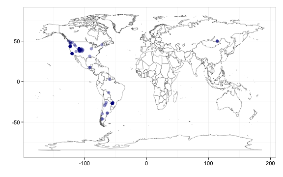
You can now map point results, from fxns occurrencelist and those from densitylist, which plots them as points or as tiles, respectively. Point map, using output from occurrencelist.
out <- occurrencelist(scientificname = "Puma concolor", coordinatestatus = TRUE,
    maxresults = 100, latlongdf = T)
gbifmap(input = out)  # make a map, plotting on world map
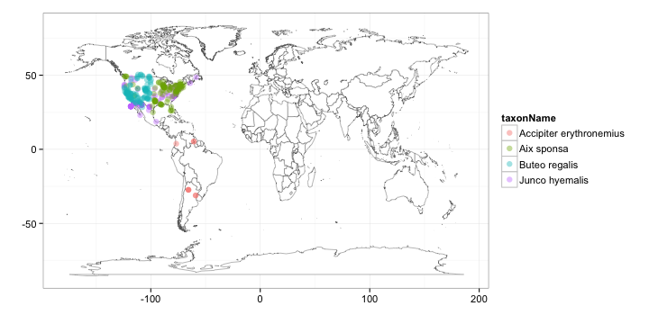
Point map, using output from occurrencelist, with many species plotted as different colors
splist <- c("Accipiter erythronemius", "Junco hyemalis", "Aix sponsa", "Buteo regalis")
out <- lapply(splist, function(x) occurrencelist(x, coordinatestatus = T, maxresults = 100,
    latlongdf = T))
gbifmap(out)
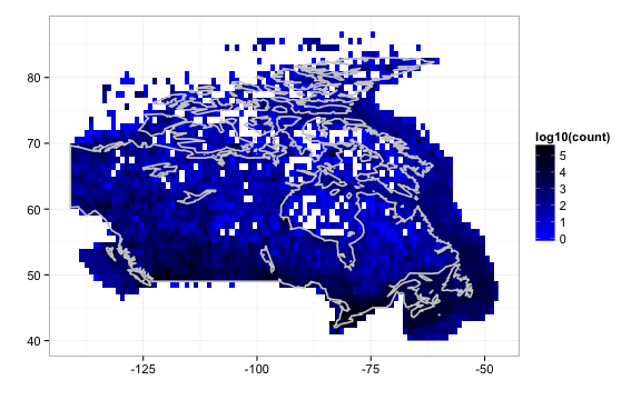
Tile map, using output from densitylist, using results in Canada only.
out2 <- densitylist(originisocountrycode = "CA")  # data for Canada
gbifmap(out2)  # on world map
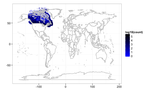
gbifmap(out2, region = "Canada") # on Canada map
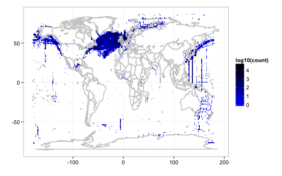
We can also query by higher taxonomic rankings, and map all lower species within that ranking. Above we queried by scientificname, but we can also query by higher taxonomy. 7071443 is the taxonconceptkey for ‘Bacillariophyceae’, a Class which includes many lower species.
out <- densitylist(taxonconceptKey = 7071443)
gbifmap(out)
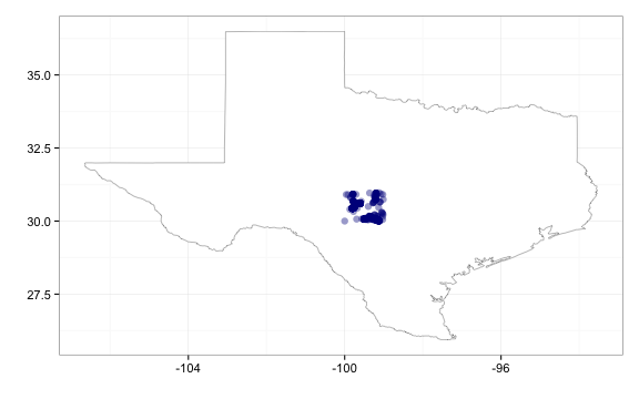
seminym asked about querying by area. You can query by area, though slightly differently for occurrencelist and densitylist functions. For occurrencelist you can search using min and max lat and long values (and min an max altitude, pretty cool, eh).
# Get occurrences or density by area, using min/max lat/long coordinates
out <- occurrencelist(minlatitude = 30, maxlatitude = 35, minlongitude = -100,
    maxlongitude = -95, coordinatestatus = T, maxresults = 5000, latlongdf = T)

# Using `geom_point`
gbifmap(out, "state", "texas", geom_point)
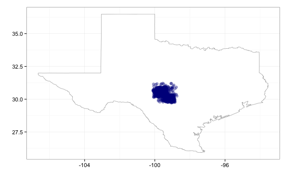
# Using geom_jitter to move the points apart from one another
gbifmap(out, "state", "texas", geom_jitter, position_jitter(width = 0.3, height = 0.3))
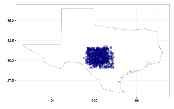
# And move points a lot
gbifmap(out, "state", "texas", geom_jitter, position_jitter(width = 1, height = 1))
And you can query by area in densitylist by specifying a place using the originisocountrycode argument (as done in an above example). Just showing the head of the data.frame here.
# Get density by place, note that you can't use the lat and long arguments
# in densitylist
head(densitylist(originisocountrycode = "CA"))
  cellid minLatitude maxLatitude minLongitude maxLongitude count
1  46913          40          41          -67          -66    44
2  46914          40          41          -66          -65   907
3  46915          40          41          -65          -64   510
4  46916          40          41          -64          -63   645
5  46917          40          41          -63          -62    56
6  46918          40          41          -62          -61   143
Get the .Rmd file used to create this post at my github account - or .md file.