I need to simulate balanced and unbalanced phylogenetic trees for some research I am doing. In order to do this, I do rejection sampling: simulate a tree -> measure tree shape -> reject if not balanced or unbalanced enough. But what is enough? We need to define some cutoff value to determine what will be our set of balanced and unbalanced trees.
calculate shape metrics
A function to calculate shape metrics, and a custom theme for plottingn phylogenies.
foo <- function(x, metric = "colless") {
    if (metric == "colless") {
        xx <- as.treeshape(x)  # convert to apTreeshape format
        colless(xx, "yule")  # calculate colless' metric
    } else if (metric == "gamma") {
        gammaStat(x)
    } else stop("metric should be one of colless or gamma")
}

theme_myblank <- function() {
    stopifnot(require(ggplot2))
    theme_blank <- ggplot2::theme_blank
    ggplot2::theme(panel.grid.major = element_blank(), panel.grid.minor = element_blank(),
        panel.background = element_blank(), plot.background = element_blank(),
        axis.title.x = element_text(colour = NA), axis.title.y = element_blank(),
        axis.text.x = element_blank(), axis.text.y = element_blank(), axis.line = element_blank(),
        axis.ticks = element_blank())
}
Simulate some trees
library(ape)
library(phytools)

numtrees <- 1000  # lets simulate 1000 trees
trees <- pbtree(n = 50, nsim = numtrees, ape = F)  # simulate 500 pure-birth trees with 100 spp each, ape = F makes it run faster
Calculate Colless’ shape metric on each tree
library(plyr)
library(apTreeshape)

colless_df <- ldply(trees, foo, metric = "colless")  # calculate metric for each tree
head(colless_df)
       V1
1 -0.1761
2  0.2839
3  0.4639
4  0.9439
5 -0.6961
6 -0.1161
# Calculate the percent of trees that will fall into the cutoff for balanced and unbalanced trees
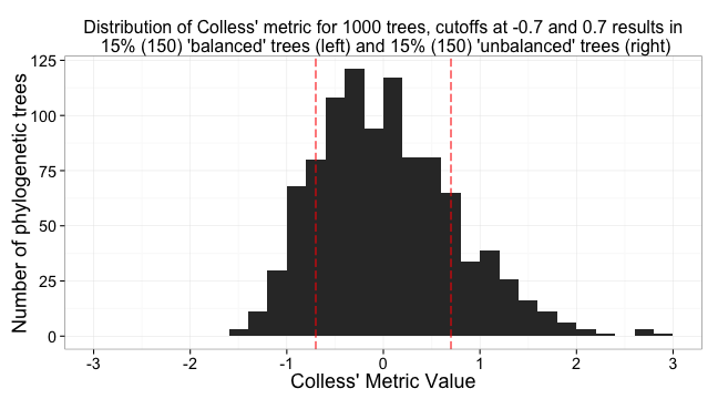
col_percent_low <- round(length(colless_df[colless_df$V1 < -0.7, "V1"])/numtrees, 2) * 100
col_percent_high <- round(length(colless_df[colless_df$V1 > 0.7, "V1"])/numtrees, 2) * 100
Create a distribution of the metric values
library(ggplot2)

a <- ggplot(colless_df, aes(V1)) +  # plot histogram of distribution of values
	geom_histogram() +
	theme_bw(base_size=18) +
	scale_x_continuous(limits=c(-3,3), breaks=c(-3,-2,-1,0,1,2,3)) +
	geom_vline(xintercept = -0.7, colour="red", linetype = "longdash") +
	geom_vline(xintercept = 0.7, colour="red", linetype = "longdash") +
	ggtitle(paste0("Distribution of Colless' metric for 1000 trees, cutoffs at -0.7 and 0.7 results in\n ", col_percent_low, "% (", numtrees*(col_percent_low/100), ") 'balanced' trees (left) and ", col_percent_low, "% (", numtrees*(col_percent_low/100), ") 'unbalanced' trees (right)")) +
	labs(x = "Colless' Metric Value", y = "Number of phylogenetic trees") +
	theme(plot.title  = element_text(size = 16))

a
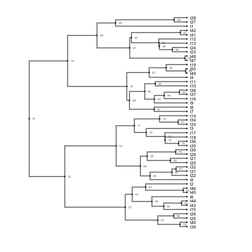
Create phylogenies representing balanced and unbalanced trees (using the custom theme)
library(ggphylo)

b <- ggphylo(trees[which.min(colless_df$V1)], do.plot = F) + theme_myblank()
c <- ggphylo(trees[which.max(colless_df$V1)], do.plot = F) + theme_myblank()

b
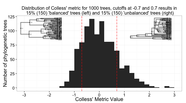
Now, put it all together in one plot using some gridExtra magic.
library(gridExtra)

grid.newpage()
pushViewport(viewport(layout = grid.layout(1, 1)))
vpa_ <- viewport(width = 1, height = 1, x = 0.5, y = 0.49)
vpb_ <- viewport(width = 0.35, height = 0.35, x = 0.23, y = 0.7)
vpc_ <- viewport(width = 0.35, height = 0.35, x = 0.82, y = 0.7)
print(a, vp = vpa_)
print(b, vp = vpb_)
print(c, vp = vpc_)
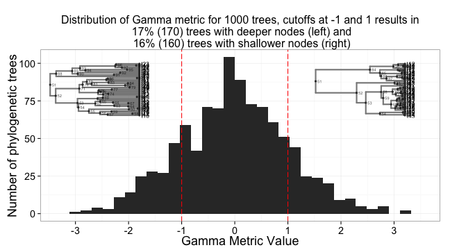
And the same for Gamma stat, which measures the distribution of nodes in time.
gamma_df <- ldply(trees, foo, metric="gamma") # calculate metric for each tree
gam_percent_low <- round(length(gamma_df[gamma_df$V1 < -1, "V1"])/numtrees, 2)*100
gam_percent_high <- round(length(gamma_df[gamma_df$V1 > 1, "V1"])/numtrees, 2)*100
a <- ggplot(gamma_df, aes(V1)) +  # plot histogram of distribution of values
	geom_histogram() +
	theme_bw(base_size=18) +
	scale_x_continuous(breaks=c(-3,-2,-1,0,1,2,3)) +
	geom_vline(xintercept = -1, colour="red", linetype = "longdash") +
	geom_vline(xintercept = 1, colour="red", linetype = "longdash") +
	ggtitle(paste0("Distribution of Gamma metric for 1000 trees, cutoffs at -1 and 1 results in\n ", gam_percent_low, "% (", numtrees*(gam_percent_low/100), ") trees with deeper nodes (left) and ", gam_percent_high, "% (", numtrees*(gam_percent_high/100), ") trees with shallower nodes (right)")) +
	labs(x = "Gamma Metric Value", y = "Number of phylogenetic trees") +
	theme(plot.title  = element_text(size = 16))
b <- ggphylo(trees[which.min(gamma_df$V1)], do.plot=F) + theme_myblank()
c <- ggphylo(trees[which.max(gamma_df$V1)], do.plot=F) + theme_myblank()

grid.newpage()
pushViewport(viewport(layout = grid.layout(1,1)))
vpa_ <- viewport(width = 1, height = 1, x = 0.5, y = 0.49)
vpb_ <- viewport(width = 0.35, height = 0.35, x = 0.23, y = 0.7)
vpc_ <- viewport(width = 0.35, height = 0.35, x = 0.82, y = 0.7)
print(a, vp = vpa_)
print(b, vp = vpb_)
print(c, vp = vpc_)
Get the .Rmd file used to create this post at my github account - or .md file.