Okay, so this isn’t ecology related at all, but I like exploring data sets. So here goes…
Propublica has some awesome data sets available at their website: http://www.propublica.org/tools/
I played around with their data set on Recovery.gov (see hyperlink below in code). Here’s some figures:
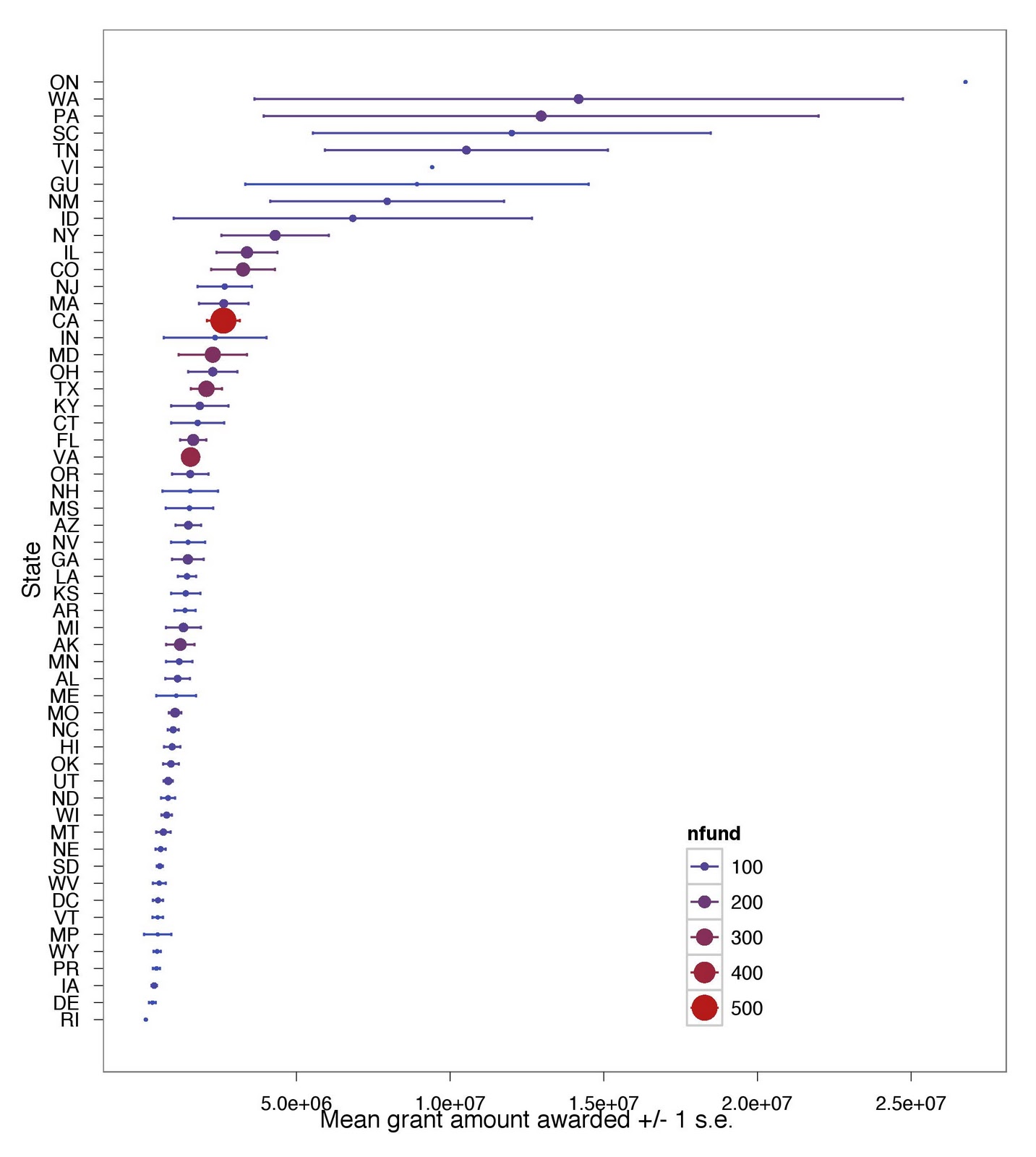
Mean award amount, ranked by mean amount, and also categorized by number of grants received (“nfund”) by state (by size and color of point). Yes, there are 56 “states”, which includes things like Northern Marian Islands (MP). Notice that California got the largest number of awards, but the mean award size was relatively small.
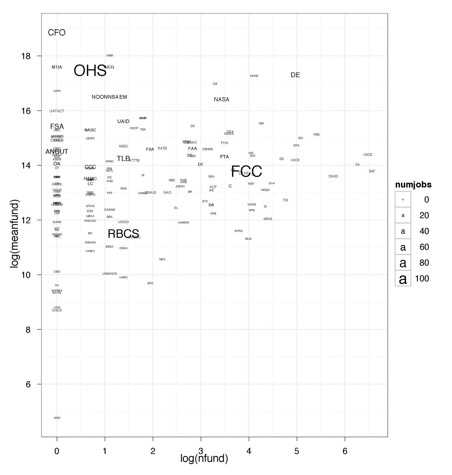
Here is a figure by government organization that awarded each award, by mean award size (y-axis), number of awards (x-axis), and number of jobs created (numjobs=text size). Notice that the FCC (Federal Communications Commission) created nearly the most jobs despite not giving very large awards (although they did give a lot of awards).
Here is the code:
# Propublica Recovery.gov data
install.packages(c("ggplot2","maps","stringr"))
library(ggplot2)
library(maps)
library(stringr)
setwd("/Mac/R_stuff/Blog_etc") # Set working directory
theme_set(theme_bw())

# Read propublica data from file (download from here: http://propublica.s3.amazonaws.com/assets/recoverygov/propublica-recoverygov-primary-2.xls
propubdat <- read.csv("propublica-recoverygov-primary-2.csv")
str(propubdat)

# Summarize data
fundbystate <- ddply(propubdat,.(prime_state),summarise,
 meanfund = mean(award_amount),
 sefund = sd(award_amount)/sqrt(length(award_amount)),
 nfund = length(award_amount),
 numjobs = mean(number_of_jobs)
)

fundbyagency <- ddply(propubdat,.(funding_agency_name),summarise,
 meanfund = mean(award_amount),
 sefund = sd(award_amount)/sqrt(length(award_amount)),
 nfund = length(award_amount),
 numjobs = mean(number_of_jobs)
)


fun1 <- function(a) {str_c(paste(na.omit(str_extract(unlist(str_split(unlist(as.character(a[1])), " ")), "[A-Z]{1}"))), collapse="")} # Fxn to make funding agency name abbreviations within ddply below

fundbyagency2 <- ddply(fundbyagency,.(funding_agency_name),transform, # add to table funding agency name abbreviations
 agency_abbrev = fun1(funding_agency_name)
)

# Plot data, means and se's by state
limits <- aes(ymax = meanfund + sefund, ymin = meanfund - sefund)
dodge <- position_dodge(width=0.6)
awardbystate <- ggplot(fundbystate,aes(x=reorder(prime_state,meanfund),y=meanfund,colour=nfund)) + geom_point(aes(size=nfund),position=dodge) + coord_flip()  + geom_errorbar(limits, width=0.2,position=dodge) + opts(panel.grid.major = theme_blank(),panel.grid.minor=theme_blank(),legend.position=c(0.7,0.2)) + labs(x="State",y="Mean grant amount awarded +/- 1 s.e.")
ggsave("awardbystate.jpeg")

# Plot data, means and se's by funding agency
limits2 <- aes(ymax = meanfund + sefund, ymin = meanfund - sefund)
dodge <- position_dodge(width=0.6)
awardbyagency <- ggplot(fundbyagency2,aes(y=log(meanfund),x=log(nfund),label=agency_abbrev)) + geom_text(aes(size=numjobs))
ggsave("awardbyagency.jpeg")


# On US map
fundbystate2 <- read.csv("fundbystate.csv")

states <- map_data("state") # get state geographic data from the maps package
recovmap <- merge(states,fundbystate2,by="region") # merage datasets

qplot(long,lat,data=recovmap,group=group,fill=meanfund,geom="polygon")
ggsave("bystatemapmeans.jpeg")

qplot(long,lat,data=recovmap,group=group,fill=nfund,geom="polygon")
ggsave("bystatemapnumber.jpeg")
And the text file fundbystate2 here. I had the make this file separately so I could get in the spelled out state names as they were not provided in the propublica dataset.
Source and disclaimer:
Data provided by Propublica. Data may contain errors and/or omissions.