[UPDATE: i remade the maps in green, hope that helps…]
A recent survey reported in Science (“Defeating Creationism in the Courtroom, but not in the Classroom”) found that biology teachers in high school do not often accept the basis of their discipline, as do teachers in other disciplines, and thus may not teach evolution appropriately. Read more here: New York Times.
I took a little time to play with the data provided online along with the Science article. The data is available on the Science website along with the article, and the dataset I read into R is unchanged from the original. The states abbreviations file is here (as a .xls). Here goes:
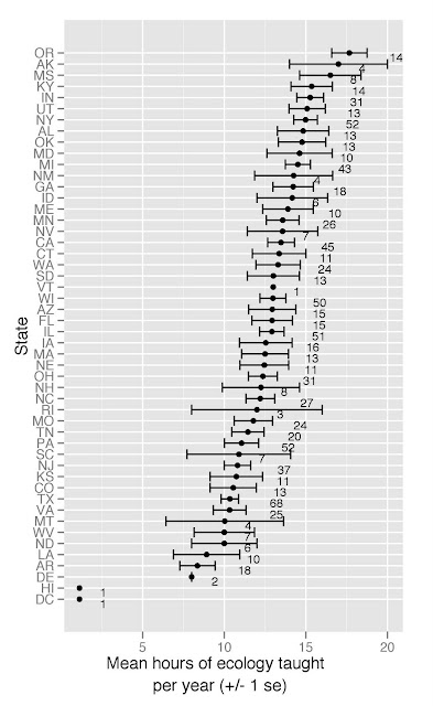
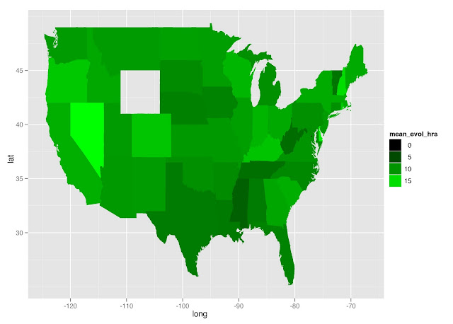
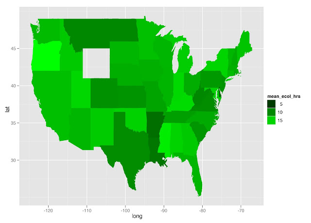
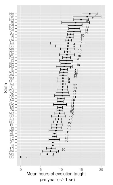
I only played with two survey questions: q1b (no. of hours ecology is taught per year), and q1d (no. of hours evolution is taught per year). I looked at ecology and evolution as this blog is about ecology and evolution. It seems that some states that teach a lot of ecology teach a lot of evolution, but I found no correlation between the two without extreme outliers. I couldn’t help but notice my home state, TX, is near the bottom of the list on both counts - go TX! The teaching of evolution on the map produced below is less predictable than I would have though just based on my assumptions about political will in each state.
# Analyses of Conditionality Data set of all variables, except for latitude, etc.
setwd("/Mac/R_stuff/Blog_etc/EvolutionTeaching/") # Set working directory
library(ggplot2)

# read in data, and prepare new columns
survey <- read.csv("berkmandata.csv")
str(survey) # (I do realize that survey is a data object in the MASS package)

# Assign actual hours to survey answers
ecol <- gsub(1, 0, survey$q1b)
ecol <- gsub(2, 1.5, ecol)
ecol <- gsub(3, 4, ecol)
ecol <- gsub(4, 8, ecol)
ecol <- gsub(5, 13, ecol)
ecol <- gsub(6, 18, ecol)
ecol <- gsub(7, 20, ecol)

evol <- gsub(1, 0, survey$q1d)
evol <- gsub(2, 1.5, evol)
evol <- gsub(3, 4, evol)
evol <- gsub(4, 8, evol)
evol <- gsub(5, 13, evol)
evol <- gsub(6, 18, evol)
evol <- gsub(7, 20, evol)

survey$ecol <- as.numeric(ecol)
survey$evol <- as.numeric(evol)

# ddply it
survey_sum <- ddply(survey, .(st_posta), summarise,
 mean_ecol_hrs = mean(ecol, na.rm=T),
 mean_evol_hrs = mean(evol, na.rm=T),
 se_ecol_hrs = sd(ecol, na.rm=T)/sqrt(length(ecol)),
 se_evol_hrs = sd(evol, na.rm=T)/sqrt(length(evol)),
 num_teachers = length(st_posta)
)

# plotting
limits_ecol <- aes(ymax = mean_ecol_hrs + se_ecol_hrs, ymin = mean_ecol_hrs - se_ecol_hrs)
limits_evol <- aes(ymax = mean_evol_hrs + se_evol_hrs, ymin = mean_evol_hrs - se_evol_hrs)

ggplot(survey_sum, aes(x = reorder(st_posta, mean_ecol_hrs), y = mean_ecol_hrs)) +
 geom_point() +
 geom_errorbar(limits_ecol) +
 geom_text(aes(label = num_teachers), vjust = 1, hjust = -3, size = 3) +
 coord_flip() +
 labs(x = "State", y = "Mean hours of ecology taught \n per year (+/- 1 se)")

####SMALL NUMBERS BY BARS ARE NUMBER OF TEACHERS THAT RESPONDED TO


