rgauges - fun with hourly web site analytics

Gaug.es is a really nice looking analytics platform as an alternative to Google Analytics. It is a paid service, but not that expensive really.

We’ve made an R package to interact with the Gaug.es API called rgauges. Find it on Github and on CRAN.

Although working with the Gaug.es API is nice and easy, they don’t keep hourly visit stats and provide those via the API, so that you have to continually collect them yourself if you want them. That’s what I have done for my own website.

It took a few steps to get this data:

I wrote a little Ruby script using Twelve gem to collect data from the Gaug.es API every day at the same time, which just gets the patst 24 hours of data. This script makes a call to the Gaug.es API and sends the data to a CouchDB database hosted on Cloudant. In reality, the script is is embeded in a rack app as I don’t think you can throw up a standalone script to Heroku. Here’s the script:

class MyApp
  require 'couchrest'
  require 'twelve'
  require 'date'
  require 'time'
  
  def self.getgaugesdata_scott
    bfg = Twelve.new('<gaugeskey>')
    out = bfg.gauges('<gaugeskey>')['recent_hours']
    yip = { "from_url"=> "http://sckott.github.io/", "coll_date"=> Date.today.to_s, "coll_time"=> Time.now.utc.localtime.to_s, "recent_hours"=> out }
    @db = CouchRest.database!("https://app16517180.heroku:<key>@app16517180.heroku.cloudant.com/gaugesdb_scott")
    @db.save_doc(yip)

  def call env
    [200, {"Content-Type" => "text/html"}, ["no output printed here"]] 
  end
end

One little catch though: I run the Ruby script on Heroku, so I don’t have to do it locally, but Heroku free instance goes down unless it’s doing something. So I used a little service called UptimeRobot to ping the Heroku app every 5 minutes. UptimeRobot also is giving you uptime stats too on your app, which I don’t really need, but is a cool feature.
And that’s it. Now the data is stored from each day’s collection of visitor stats to a free Cloudant CouchDB database.

Regular Gaug.es data

First, let’s look at what you can do with data that Gaug.es does give to you, using the rgauges R package.

Install rgauges

install.packages("devtools")
library(devtools)
install_github("rgauges", "ropensci")

Load rgauges and other dependency libraries

library(rgauges)
library(ggplot2)

Your info

gs_me()

## $user
## $user$name
## [1] "Scott Chamberlain"
## 
## $user$email
## [1] "myrmecocystus@gmail.com"
## 
## $user$id
## [1] "4eddbafb613f5d5139000001"
## 
## $user$last_name
## [1] "Chamberlain"
## 
## $user$urls
## $user$urls$self
## [1] "https://secure.gaug.es/me"
## 
## $user$urls$clients
## [1] "https://secure.gaug.es/clients"
## 
## $user$urls$gauges
## [1] "https://secure.gaug.es/gauges"
## 
## 
## $user$first_name
## [1] "Scott"

Traffic

gs_traffic(id = "4efd83a6f5a1f5158a000004")

## $metadata
## $metadata$views
## [1] 386
## 
## $metadata$urls
## $metadata$urls$older
## [1] "https://secure.gaug.es/gauges/4efd83a6f5a1f5158a000004/traffic?date=2013-12-01"
## 
## $metadata$urls$newer
## NULL
## 
## 
## $metadata$date
## [1] "2014-01-17"
## 
## $metadata$people
## [1] 208
## 
## 
## $data
##    views       date people
## 1      7 2014-01-01      5
## 2     17 2014-01-02      7
## 3     39 2014-01-03     17
## 4     15 2014-01-04      9
## 5     14 2014-01-05      7
## 6     33 2014-01-06     22
## 7     19 2014-01-07     11
## 8     15 2014-01-08     11
## 9     53 2014-01-09     24
## 10    53 2014-01-10     13
## 11    14 2014-01-11      9
## 12    11 2014-01-12     10
## 13    14 2014-01-13     14
## 14    11 2014-01-14      9
## 15    23 2014-01-15     16
## 16    16 2014-01-16     14
## 17    32 2014-01-17     25

Screen/browser information

gs_reso(id = "4efd83a6f5a1f5158a000004")

## $browser_height
##   views title
## 1   190   600
## 2    77   768
## 3    53   900
## 4    38   480
## 5    28  1024
## 
## $browser_width
##   views title
## 1   153  1280
## 2    91  1024
## 3    58  1600
## 4    36   800
## 5    30  1440
## 6     6  2000
## 7     6   320
## 8     6   480
## 
## $screen_width
##   views title
## 1   176  1280
## 2    90  1600
## 3    55  1440
## 4    35  1024
## 5    14  2000
## 6     6   320
## 7     6   480
## 8     4   800

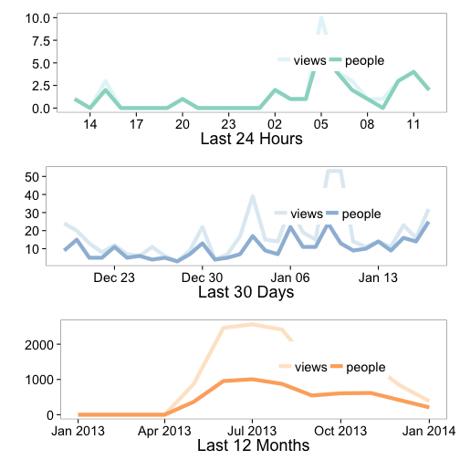
Visualize traffic data

You’ll need to load ggplot2

library(ggplot2)
out <- gs_gauge_detail(id = "4efd83a6f5a1f5158a000004")
vis_gauge(out)

## Using hour, time as id variables
## Using date as id variables
## Using date as id variables

center

## NULL

Historic hourly Gaug.es data

Now let’s play with the hourly data. To do that we aren’t going to use rgauges, but rather call the Cloudant API. CouchDB provides a RESTful API out of the box, so we can do a call like https://app16517180.heroku.cloudant.com/gaugesdb_scott/_all_docs?limit=20 to get metadata (or other calls to get the documents themselves). (note: that url won’t work for you since you don’t have my login info)

Get some data

library(devtools)
install_github("sckott/sofa")  # or install_github('sofa', 'sckott')

library(sofa)
cloudant_name <- "app16517180.heroku"
cloudant_pwd <- getOption("sofa_cloudant_heroku")[[2]]
cushion(sofa_cloudant = c(cloudant_name, cloudant_pwd))
dat <- sofa_alldocs(cushion = "sofa_cloudant", dbname = "gaugesdb_scott", include_docs = "true")

Manipulate and visualize

library(plyr)
dates <- ldply(dat$rows, function(x) x$doc$coll_date)
min(dates$V1)

## [1] "2013-06-26"

max(dates$V1)

## [1] "2014-01-16"

length(dates$V1)

## [1] 198

So we’ve got 198 days of data, first collected near end of June, and most recent yesterday. Now get actual visits data

df <- ldply(dat$rows, function(x) {
    y <- do.call(rbind, lapply(x$doc$recent_hours, data.frame))
    data.frame(date = x$doc$coll_date, y)
})
df$date <- as.Date(df$date)
df$hour <- as.numeric(df$hour)

library(reshape2)
df_melt <- melt(df, id.vars = c("date", "hour"))
head(df_melt)

##         date hour variable value
## 1 2013-09-18    1    views     2
## 2 2013-09-18    2    views     3
## 3 2013-09-18    3    views     2
## 4 2013-09-18    4    views     0
## 5 2013-09-18    5    views     1
## 6 2013-09-18    6    views    10

We need to combine the date and hour in to one date time string:

df_melt <- transform(df_melt, datetime = as.POSIXct(paste(date, sprintf("%s:00:00", 
    hour))))
head(df_melt)

##         date hour variable value            datetime
## 1 2013-09-18    1    views     2 2013-09-18 01:00:00
## 2 2013-09-18    2    views     3 2013-09-18 02:00:00
## 3 2013-09-18    3    views     2 2013-09-18 03:00:00
## 4 2013-09-18    4    views     0 2013-09-18 04:00:00
## 5 2013-09-18    5    views     1 2013-09-18 05:00:00
## 6 2013-09-18    6    views    10 2013-09-18 06:00:00

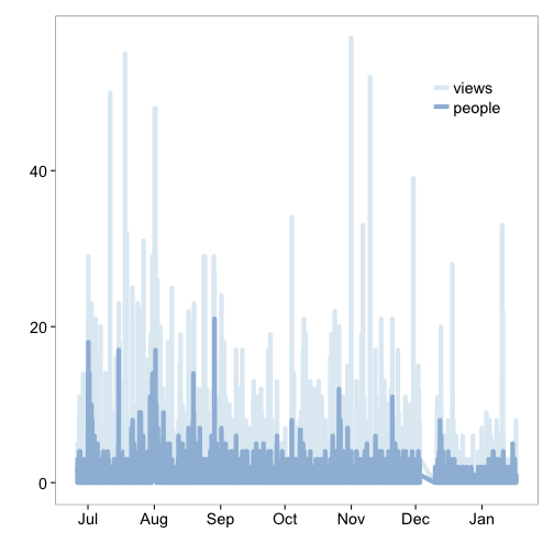
Now plot all data

library(ggplot2); library(scales)

gauge_theme <- function(){
  list(theme(panel.grid.major = element_blank(),
             panel.grid.minor = element_blank(),
             legend.position = c(0.85,0.85),
             legend.key = element_blank()))
}

ggplot(df_melt, aes(datetime, value, group=variable, colour=variable)) +
    theme_bw(base_size=18) + 
    geom_line(size=2) +
    scale_color_brewer(name="", palette=3) +
    labs(x="", y="") +
    gauge_theme()

center

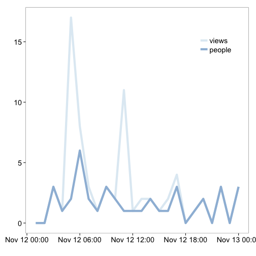
And just one day

oneday <- df_melt[ as.character(df_melt$date) %in% "2013-11-12", ]
ggplot(oneday, aes(datetime, value, group=variable, colour=variable)) +
    theme_bw(base_size=18) + 
    geom_line(size=2) +
    scale_color_brewer(name="", palette=3) +
    labs(x="", y="") +
    gauge_theme()

center

Regular Gaug.es data#

Install rgauges#

Load rgauges and other dependency libraries#

Your info#

Traffic#

Screen/browser information#

Visualize traffic data#

Historic hourly Gaug.es data#

Get some data#

Manipulate and visualize#

Regular Gaug.es data

Install rgauges

Load rgauges and other dependency libraries

Your info

Traffic

Screen/browser information

Visualize traffic data

Historic hourly Gaug.es data

Get some data

Manipulate and visualize