Someone asked about plotting something like this today
I wrote a few functions previously to do something like this. However, since then ggplot2 has changed, and one of the functions no longer works.
Hence, I fixed opts() to theme(), theme_blank() to element_blank(), and panel.background = element_blank() to plot.background = element_blank() to get the histograms to show up with the line plot and not cover it.
The new functions:
loghistplot  <- function(data) {
  names(data) <- c('x','y') # rename columns

  # get min and max axis values
  min_x <- min(data$x)
  max_x <- max(data$x)
  min_y <- min(data$y)
  max_y <- max(data$y)

  # get bin numbers
  bin_no <- max(hist(data$x, plot = FALSE)$counts) + 5

  # create plots
  a <- ggplot(data, aes(x = x, y = y)) +
    theme_bw(base_size=16) +
    geom_smooth(method = "glm", family = "binomial", se = TRUE,
                colour='black', size=1.5, alpha = 0.3) +
    scale_x_continuous(limits=c(min_x,max_x)) +
    theme(panel.grid.major = element_blank(),
          panel.grid.minor=element_blank(),
          panel.background = element_blank(),
          plot.background = element_blank()) +
    labs(y = "Probability\n", x = "\nYour X Variable")

  theme_loghist <- list(
    theme(panel.grid.major = element_blank(),
          panel.grid.minor=element_blank(),
          axis.text.y = element_blank(),
          axis.text.x = element_blank(),
          axis.ticks = element_blank(),
          panel.border = element_blank(),
          panel.background = element_blank(),
          plot.background = element_blank())
  )

  b <-
  ggplot(data[data$y == unique(data$y)[1], ], aes(x = x)) +
    theme_bw(base_size=16) +
    geom_histogram(fill = "grey") +
    scale_y_continuous(limits=c(0,bin_no)) +
    scale_x_continuous(limits=c(min_x,max_x)) +
    theme_loghist +
    labs(y='\n', x='\n')

  c <- ggplot(data[data$y == unique(data$y)[2], ], aes(x = x)) +
    theme_bw(base_size=16) +
    geom_histogram(fill = "grey") +
    scale_y_continuous(trans='reverse', limits=c(bin_no,0)) +
    scale_x_continuous(limits=c(min_x,max_x)) +
    theme_loghist +
    labs(y='\n', x='\n')

  grid.newpage()
  pushViewport(viewport(layout = grid.layout(1,1)))

  vpa_ <- viewport(width = 1, height = 1, x = 0.5, y = 0.5)
  vpb_ <- viewport(width = 1, height = 1, x = 0.5, y = 0.5)
  vpc_ <- viewport(width = 1, height = 1, x = 0.5, y = 0.5)

  print(b, vp = vpb_)
  print(c, vp = vpc_)
  print(a, vp = vpa_)
}
logpointplot  <- function(data) {
  names(data) <- c('x','y') # rename columns

  # get min and max axis values
  min_x <- min(data$x)
  max_x <- max(data$x)
  min_y <- min(data$y)
  max_y <- max(data$y)

  # create plots
  ggplot(data, aes(x = x, y = y)) +
    theme_bw(base_size=16) +
    geom_point(size = 3, alpha = 0.5, position = position_jitter(w=0, h=0.02)) +
    geom_smooth(method = "glm", family = "binomial", se = TRUE,
                colour='black', size=1.5, alpha = 0.3) +
    scale_x_continuous(limits=c(min_x,max_x)) +
    theme(panel.grid.major = element_blank(),
          panel.grid.minor=element_blank(),
          panel.background = element_blank()) +
    labs(y = "Probability\n", x = "\nYour X Variable")

}
Install ggplot2 and gridExtra if you don’t have them:
install.packages(c("ggplot2","gridExtra"), repos = "http://cran.rstudio.com")
And their use:
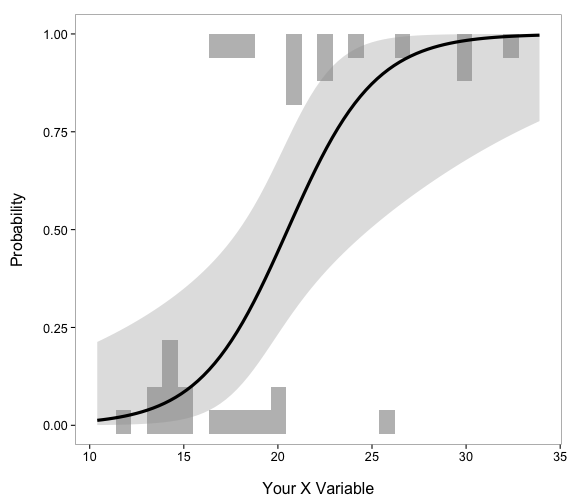
Logistic histogram plots
loghistplot(data=mtcars[,c("mpg","vs")])
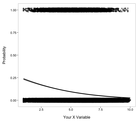
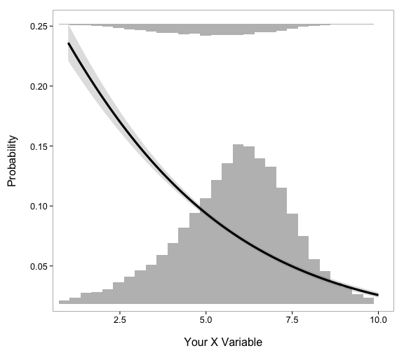
loghistplot(movies[,c("rating","Action")])
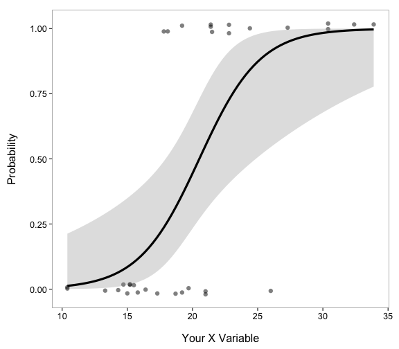
Logistic point plots
loghistplot(data=mtcars[,c("mpg","vs")])
loghistplot(movies[,c("rating","Action")])