lawn is an R wrapper for the Javascript library turf.js for advanced geospatial analysis. In addition, we have a few functions to interface with the geojson-random Javascript library.
lawn includes traditional spatial operations, helper functions for creating GeoJSON data, and data classification and statistics tools.
There is an additional helper function (see view()) in this package to help visualize data with interactive maps via the leaflet package (https://github.com/rstudio/leaflet). Note that leaflet is not required to install lawn - it’s in Suggests, not Imports or Depends.
Use cases for this package include (but not limited to, obs.) the following (all below assumes GeoJSON format):
- Create random spatial data.
- Convert among spatial data types (e.g.
PolygontoFeatureCollection) - Transform objects, including merging many, simplifying, calculating hulls, etc.
- Measuring objects
- Performing interpolation of objects
- Aggregating data (aka properties) associated with objects
Install
Stable lawn version from CRAN - this should fetch leaflet, which is not on CRAN, but in a drat repo (let me know if it doesn’t)
install.packages("lawn")
Or, the development version from Github
devtools::install_github("ropensci/lawn")
library("lawn")
view
lawn includes a tiny helper function for visualizing geojson. For examples below, we’ll make liberal use of the lawn::view() function to visualize what it is the heck we’re doing. mkay, lets roll…
We’ve tried to make view() work with as many inputs as possible, from class character containing
json to the class json from the jsonlite package, to the class list to all of the GeoJSON outputs
from functions in lawn.
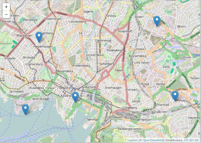
view(lawn_data$points_average)
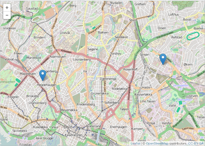
Here, we sample at random two points from the same dataset just viewed.
lawn_sample(lawn_data$points_average, 2) %>% view()
Make some geojson data
Point
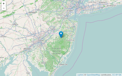
lawn_point(c(-74.5, 40))
#> $type
#> [1] "Feature"
#>
#> $geometry
#> $geometry$type
#> [1] "Point"
#>
#> $geometry$coordinates
#> [1] -74.5  40.0
#>
#>
#> $properties
#> named list()
#>
#> attr(,"class")
#> [1] "point"
lawn_point(c(-74.5, 40)) %>% view
Polygon
rings <- list(list(
c(-2.275543, 53.464547),
c(-2.275543, 53.489271),
c(-2.215118, 53.489271),
c(-2.215118, 53.464547),
c(-2.275543, 53.464547)
))
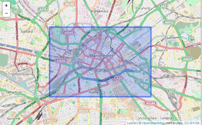
lawn_polygon(rings)
#> $type
#> [1] "Feature"
#>
#> $geometry
#> $geometry$type
#> [1] "Polygon"
#>
#> $geometry$coordinates
#> , , 1
#>
#> [,1] [,2] [,3] [,4] [,5]
#> [1,] -2.275543 -2.275543 -2.215118 -2.215118 -2.275543
#>
#> , , 2
#>
#> [,1] [,2] [,3] [,4] [,5]
#> [1,] 53.46455 53.48927 53.48927 53.46455 53.46455
#>
#>
#>
#> $properties
#> named list()
#>
#> attr(,"class")
#> [1] "polygon"
lawn_polygon(rings) %>% view
Random set of points
lawn_random(n = 2)
#> $type
#> [1] "FeatureCollection"
#>
#> $features
#>      type geometry.type  geometry.coordinates
#> 1 Feature         Point -137.46327, -63.46154
#> 2 Feature         Point  -110.68426, 83.10533
#>
#> attr(,"class")
#> [1] "featurecollection"
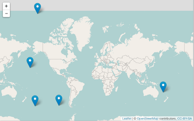
lawn_random(n = 5) %>% view
Or, use a different Javascript library (geojson-random) to create random features.
Positions
gr_position()
#> [1] -179.77996   45.99018
Points
gr_point(2)
#> $type
#> [1] "FeatureCollection"
#>
#> $features
#>      type geometry.type geometry.coordinates
#> 1 Feature         Point   5.83895, -27.77218
#> 2 Feature         Point   78.50177, 14.95840
#>
#> attr(,"class")
#> [1] "featurecollection"
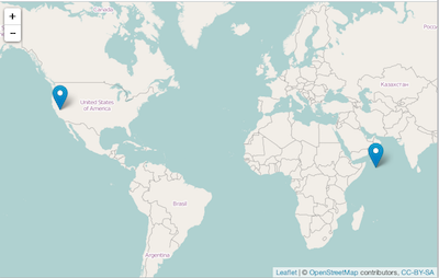
gr_point(2) %>% view
Polygons
gr_polygon(n = 1, vertices = 5, max_radial_length = 5)
#> $type
#> [1] "FeatureCollection"
#>
#> $features
#>      type geometry.type
#> 1 Feature       Polygon
#>                                                                                                           geometry.coordinates
#> 1 67.58827, 67.68551, 67.00091, 66.70156, 65.72578, 67.58827, -42.11340, -42.69850, -43.54866, -42.42758, -41.76731, -42.11340
#>
#> attr(,"class")
#> [1] "featurecollection"
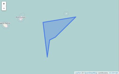
gr_polygon(n = 1, vertices = 5, max_radial_length = 5) %>% view
count
Count number of points within polygons, appends a new field to properties (see the count field)
lawn_count(polygons = lawn_data$polygons_count, points = lawn_data$points_count)
#> $type
#> [1] "FeatureCollection"
#>
#> $features
#>      type pt_count geometry.type
#> 1 Feature        2       Polygon
#> 2 Feature        0       Polygon
#>                                                                                           geometry.coordinates
#> 1 -112.07239, -112.07239, -112.02810, -112.02810, -112.07239, 46.58659, 46.61761, 46.61761, 46.58659, 46.58659
#> 2 -112.02398, -112.02398, -111.96613, -111.96613, -112.02398, 46.57043, 46.61502, 46.61502, 46.57043, 46.57043
#>
#> attr(,"class")
#> [1] "featurecollection"
distance
Define two points
from <- '{
 "type": "Feature",
 "properties": {},
 "geometry": {
   "type": "Point",
   "coordinates": [-75.343, 39.984]
 }
}'
to <- '{
  "type": "Feature",
  "properties": {},
  "geometry": {
    "type": "Point",
    "coordinates": [-75.534, 39.123]
  }
}'
Calculate distance, default units is kilometers (default output: km)
lawn_distance(from, to)
#> [1] 97.15958
sample from a FeatureCollection
dat <- lawn_data$points_average
cat(dat)
#> {
#>   "type": "FeatureCollection",
#>   "features": [
#>     {
#>       "type": "Feature",
#>       "properties": {
#>         "population": 200
#>       },
#>       "geometry": {
#>         "type": "Point",
...
Sample 2 points at random
lawn_sample(dat, 2)
#> $type
#> [1] "FeatureCollection"
#>
#> $features
#>      type population geometry.type geometry.coordinates
#> 1 Feature        200         Point   10.80643, 59.90891
#> 2 Feature        600         Point   10.71579, 59.90478
#>
#> attr(,"class")
#> [1] "featurecollection"
extent
Calculates the extent of all input features in a FeatureCollection, and returns a bounding box.
lawn_extent(lawn_data$points_average)
#> [1] 10.71579 59.90478 10.80643 59.93162
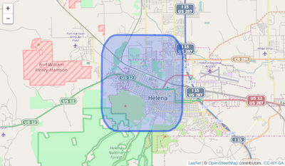
buffer
Calculates a buffer for input features for a given radius.
dat <- '{
 "type": "Feature",
 "properties": {},
 "geometry": {
     "type": "Polygon",
     "coordinates": [[
       [-112.072391,46.586591],
       [-112.072391,46.61761],
       [-112.028102,46.61761],
       [-112.028102,46.586591],
       [-112.072391,46.586591]
     ]]
   }
}'
view(dat)
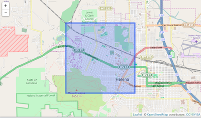
lawn_buffer(dat, 1, "miles") %>% view
Union polygons together
poly1 <- '{
 "type": "Feature",
 "properties": {
   "fill": "#0f0"
 },
 "geometry": {
   "type": "Polygon",
   "coordinates": [[
     [-122.801742, 45.48565],
     [-122.801742, 45.60491],
     [-122.584762, 45.60491],
     [-122.584762, 45.48565],
     [-122.801742, 45.48565]
    ]]
 }
}'

poly2 <- '{
 "type": "Feature",
 "properties": {
   "fill": "#00f"
 },
 "geometry": {
   "type": "Polygon",
   "coordinates": [[
     [-122.520217, 45.535693],
     [-122.64038, 45.553967],
     [-122.720031, 45.526554],
     [-122.669906, 45.507309],
     [-122.723464, 45.446643],
     [-122.532577, 45.408574],
     [-122.487258, 45.477466],
     [-122.520217, 45.535693]
     ]]
 }
}'
view(poly1)
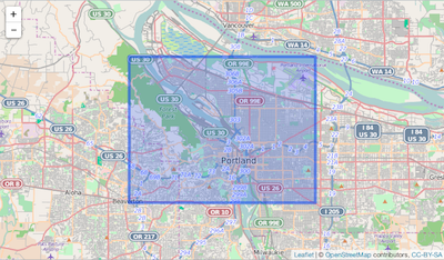
view(poly2)
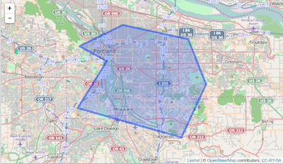
Visualize union-ed polygons
lawn_union(poly1, poly2) %>% view
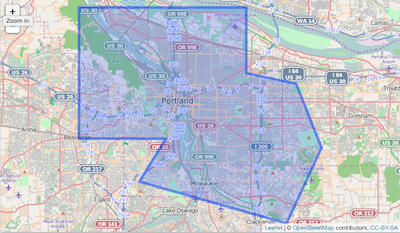
See also lawn_merge() and lawn_intersect().
lint input geojson
For most functions, you can lint your input geojson data to make sure it is proper geojson. We use
the javascript library geojsonhint. See the lint parameter.
Good GeoJSON
dat <- '{
  "type": "FeatureCollection",
  "features": [
    {
      "type": "Feature",
      "properties": {
        "population": 200
      },
      "geometry": {
        "type": "Point",
        "coordinates": [10.724029, 59.926807]
      }
    }
  ]
}'
lawn_extent(dat)
#> [1] 10.72403 59.92681 10.72403 59.92681
Bad GeoJSON
dat <- '{
  "type": "FeatureCollection",
  "features": [
    {
      "type": "Feature",
      "properties": {
        "population": 200
      },
      "geometry": {
        "type": "Point"
      }
    }
  ]
}'
lawn_extent(dat, lint = TRUE)

#> Error: Line 1 - "coordinates" property required
To do
- As Turf.js changes, we’ll update
lawn - Performance improvements. We realize that this package is slower than the C based
rgdal/rgeos- we are looking into ways to increaes performance to get closer to the performance of those packages.