iDigBio, or Integrated Digitized Biocollections, collects and provides access to species occurrence data, and associated metadata (e.g., images of specimens, when provided). They collect data from a lot of different providers. They have a nice web interface for searching, check out idigbio.org/portal/search.
spocc is a package we’ve been working on at rOpenSci for a while now - it is a one stop shop for retrieving species ocurrence data. As new sources of species occurrence data come to our attention, and are available via a RESTful API, we incorporate them into spocc.
I attended last week a hackathon put on by iDigBio. One of the projects I worked on was integrating iDigBio into spocc.
With the addition of iDigBio, we now have in spocc:
The following is a quick demo of getting iDigBio data in spocc
Install
Get updated versions of rgbif and ridigbio first. And get leaflet to make an interactive map.
devtools::install_github("ropensci/rgbif", "iDigBio/ridigbio", "rstudio/leaflet")
devtools::install_github("ropensci/spocc")
library("spocc")
Use ridigbio - the R client for iDigBio
library("ridigbio")
idig_search_records(rq = list(genus = "acer"), limit = 5)
#>                                   uuid
#> 1 00041678-5df1-4a23-ba78-8c12f60af369
#> 2 00072caf-0f24-447f-b68e-a20299f6afc7
#> 3 000a6b9b-0bbd-46f6-82cb-848c30c46313
#> 4 001d05e0-9c86-466d-957d-e73e2ce64fbe
#> 5 0022a2da-bc97-4bef-b2a5-b8a9944fc677
#>                                    occurrenceid catalognumber      family
#> 1 urn:uuid:b275f928-5c0d-4832-ae82-fde363d8fde1          <NA> sapindaceae
#> 2          40428b90-27a5-11e3-8d47-005056be0003   lsu00049997   aceraceae
#> 3          02ca5aae-d8ab-492f-af10-e005b96c2295        191243 sapindaceae
#> 4                     urn:catalog:cas:ds:679715      ds679715 sapindaceae
#> 5          b12bd651-2c6b-11e3-b3b8-180373cac83e         41898 sapindaceae
#>   genus  scientificname       country stateprovince geopoint.lat
#> 1  acer     acer rubrum united states      illinois         <NA>
#> 2  acer    acer negundo united states     louisiana         <NA>
#> 3  acer            <NA> united states      new york         <NA>
#> 4  acer acer circinatum united states    california      41.8714
#> 5  acer     acer rubrum united states      maryland   39.4197222
#>   geopoint.lon             datecollected           collector
#> 1         <NA> 1967-06-25T00:00:00+00:00     john e. ebinger
#> 2         <NA> 1991-04-19T00:00:00+00:00     alan w. lievens
#> 3         <NA>                      <NA> stephen f. hilfiker
#> 4    -123.8503 1930-10-27T00:00:00+00:00        carl b. wolf
#> 5  -77.1227778 1980-04-29T00:00:00+00:00         doweary, d.
Use spocc
Scientific name search
Same search as above with ridigbio
occ(query = "Acer", from = "idigbio", limit = 5)
#> Searched: idigbio
#> Occurrences - Found: 379, Returned: 5
#> Search type: Scientific
#>   idigbio: Acer (5)
Geographic search
iDigBio uses Elasticsearch syntax to define a geographic search, but all you need to do is give a numeric vector of length 4 defining a bounding box, and you’re good to go.
bounds <- c(-120, 40, -100, 45)
occ(from = "idigbio", geometry = bounds, limit = 10)
#> Searched: idigbio
#> Occurrences - Found: 346,737, Returned: 10
#> Search type: Geometry
W/ or W/O Coordinates
Don’t pass has_coords (gives data w/ and w/o coordinates data)
occ(query = "Acer", from = "idigbio", limit = 5)
#> Searched: idigbio
#> Occurrences - Found: 379, Returned: 5
#> Search type: Scientific
#>   idigbio: Acer (5)
Only records with coordinates data
occ(query = "Acer", from = "idigbio", limit = 5, has_coords = TRUE)
#> Searched: idigbio
#> Occurrences - Found: 16, Returned: 5
#> Search type: Scientific
#>   idigbio: Acer (5)
Only records without coordinates data
occ(query = "Acer", from = "idigbio", limit = 5, has_coords = FALSE)
#> Searched: idigbio
#> Occurrences - Found: 363, Returned: 5
#> Search type: Scientific
#>   idigbio: Acer (5)
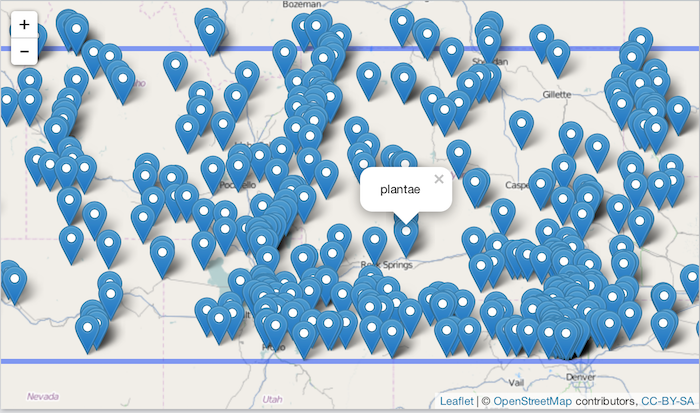
Make an interactive map
library("leaflet")
bounds <- c(-120, 40, -100, 45)
leaflet(data = dat) %>%
  addTiles() %>%
  addMarkers(~longitude, ~latitude, popup = ~name) %>%
  addRectangles(
    lng1 = bounds[1], lat1 = bounds[4],
    lng2 = bounds[3], lat2 = bounds[2],
    fillColor = "transparent"
  )