ERDDAP is a data server that gives you a simple, consistent way to download subsets of gridded and tabular scientific datasets in common file formats and make graphs and maps. Besides it’s own RESTful interface, much of which is designed based on OPeNDAP, ERDDAP can act as an OPeNDAP server and as a WMS server for gridded data.
ERDDAP is a powerful tool - in a world of heterogeneous data, it’s often hard to combine data and serve it through the same interface, with tools for querying/filtering/subsetting the data. That is exactly what ERDDAP does. Heterogeneous data sets often have some similarities, such as latitude/longitude data and usually a time component, but other variables vary widely.
NetCDF
rerddap supports NetCDF format, and is the default when using the griddap() function. We use ncdf by default, but you can choose to use ncdf4 instead.
Caching
Data files downloaded are cached in a single hidden directory ~/.rerddap on your machine. It’s hidden so that you don’t accidentally delete the data, but you can still easily delete the data if you like, open files, move them around, etc.
When you use griddap() or tabledap() functions, we construct a MD5 hash from the base URL, and any query parameters - this way each query is separately cached. Once we have the hash, we look in ~/.rerddap for a matching hash. If there’s a match we use that file on disk - if no match, we make a http request for the data to the ERDDAP server you specify.
ERDDAP servers
You can get a data.frame of ERDDAP servers using the function servers(). Most I think serve some kind of NOAA data, but there are a few that aren’t NOAA data. Here are a few:
head(servers())
#>                                                                                            name
#> 1                                                         Marine Domain Awareness (MDA) - Italy
#> 2                                                                    Marine Institute - Ireland
#> 3                                                      CoastWatch Caribbean/Gulf of Mexico Node
#> 4                                                                    CoastWatch West Coast Node
#> 5                    NOAA IOOS CeNCOOS (Central and Northern California Ocean Observing System)
#> 6 NOAA IOOS NERACOOS (Northeastern Regional Association of Coastal and Ocean Observing Systems)
#>                                        url
#> 1 https://bluehub.jrc.ec.europa.eu/erddap/
#> 2          https://erddap.marine.ie/erddap/
#> 3      https://cwcgom.aoml.noaa.gov/erddap/
#> 4  https://coastwatch.pfeg.noaa.gov/erddap/
#> 5    https://erddap.axiomalaska.com/erddap/
#> 6          https://www.neracoos.org/erddap/
Install
From CRAN
install.packages("rerddap")
Or development version from GitHub
devtools::install_github("ropensci/rerddap")
library('rerddap')
Search
First, you likely want to search for data, specifying whether to search for either griddadp or tabledap datasets. The default is griddap.
ed_search(query = 'size', which = "table")
#> 11 results, showing first 20
#>                                                                                         title
#> 1                                                                          CalCOFI Fish Sizes
#> 2                                                                        CalCOFI Larvae Sizes
#> 3                Channel Islands, Kelp Forest Monitoring, Size and Frequency, Natural Habitat
#> 4                                                         CalCOFI Larvae Counts Positive Tows
#> 5                                                                                CalCOFI Tows
#> 7                                                  OBIS - ARGOS Satellite Tracking of Animals
#> 8                                                     GLOBEC NEP MOCNESS Plankton (MOC1) Data
#> 9                                                 GLOBEC NEP Vertical Plankton Tow (VPT) Data
#> 10                            NWFSC Observer Fixed Gear Data, off West Coast of US, 2002-2006
#> 11                                 NWFSC Observer Trawl Data, off West Coast of US, 2002-2006
#> 12 AN EXPERIMENTAL DATASET: Underway Sea Surface Temperature and Salinity Aboard the Oleander
#>             dataset_id
#> 1     erdCalCOFIfshsiz
#> 2     erdCalCOFIlrvsiz
#> 3       erdCinpKfmSFNH
#> 4  erdCalCOFIlrvcntpos
#> 5       erdCalCOFItows
#> 7            aadcArgos
#> 8        erdGlobecMoc1
#> 9         erdGlobecVpt
#> 10  nwioosObsFixed2002
#> 11  nwioosObsTrawl2002
#> 12            nodcPJJU
ed_search(query = 'size', which = "grid")
#> 6 results, showing first 20
#>                                                                                                   title
#> 6                                                       NOAA Global Coral Bleaching Monitoring Products
#> 13        USGS COAWST Forecast, US East Coast and Gulf of Mexico (Experimental) [time][eta_rho][xi_rho]
#> 14            USGS COAWST Forecast, US East Coast and Gulf of Mexico (Experimental) [time][eta_u][xi_u]
#> 15            USGS COAWST Forecast, US East Coast and Gulf of Mexico (Experimental) [time][eta_v][xi_v]
#> 16 USGS COAWST Forecast, US East Coast and Gulf of Mexico (Experimental) [time][s_rho][eta_rho][xi_rho]
#> 17  USGS COAWST Forecast, US East Coast and Gulf of Mexico (Experimental) [time][Nbed][eta_rho][xi_rho]
#>             dataset_id
#> 6             NOAA_DHW
#> 13 whoi_ed12_89ce_9592
#> 14 whoi_61c3_0b5d_cd61
#> 15 whoi_62d0_9d64_c8ff
#> 16 whoi_7dd7_db97_4bbe
#> 17 whoi_a4fb_2c9c_16a7
This gives back dataset titles and identifiers - with which you should be able to get a sense for which dataset you may want to fetch.
Information
After searching you can get more information on a single dataset
info('whoi_62d0_9d64_c8ff')
#> <ERDDAP info> whoi_62d0_9d64_c8ff
#>  Dimensions (range):
#>      time: (2012-06-25T01:00:00Z, 2015-06-24T00:00:00Z)
#>      eta_v: (0, 334)
#>      xi_v: (0, 895)
#>  Variables:
#>      bedload_Vsand_01:
#>          Units: kilogram meter-1 s-1
#>      bedload_Vsand_02:
#>          Units: kilogram meter-1 s-1
...
Which is a simple S3 list but prints out pretty, so it’s easy to quickly scan the printed output and see what you need to see to proceed. That is, in the next step you want to get the dataset, and you’ll want to specify your search using some combination of values for latitude, longitude, and time.
griddap (gridded) data
First, get information on a dataset to see time range, lat/long range, and variables.
(out <- info('noaa_esrl_027d_0fb5_5d38'))
#> <ERDDAP info> noaa_esrl_027d_0fb5_5d38
#>  Dimensions (range):
#>      time: (1850-01-01T00:00:00Z, 2014-05-01T00:00:00Z)
#>      latitude: (87.5, -87.5)
#>      longitude: (-177.5, 177.5)
#>  Variables:
#>      air:
#>          Range: -20.9, 19.5
#>          Units: degC
Then query for gridded data using the griddap() function
(res <- griddap(out,
  time = c('2012-01-01', '2012-01-30'),
  latitude = c(21, 10),
  longitude = c(-80, -70)
))
#> <ERDDAP griddap> noaa_esrl_027d_0fb5_5d38
#>    Path: [~/.rerddap/648ed11e8b911b65e39eb63c8df339df.nc]
#>    Last updated: [2015-05-09 08:31:10]
#>    File size:    [0 mb]
#>    Dimensions (dims/vars):   [3 X 1]
#>    Dim names: time, latitude, longitude
#>    Variable names: CRUTEM3: Surface Air Temperature Monthly Anomaly
#>    data.frame (rows/columns):   [18 X 4]
#>                    time latitude longitude  air
#> 1  2012-01-01T00:00:00Z     22.5     -77.5   NA
#> 2  2012-01-01T00:00:00Z     22.5     -77.5   NA
#> 3  2012-01-01T00:00:00Z     22.5     -77.5   NA
#> 4  2012-01-01T00:00:00Z     22.5     -77.5 -0.1
#> 5  2012-01-01T00:00:00Z     22.5     -77.5   NA
#> 6  2012-01-01T00:00:00Z     22.5     -77.5 -0.2
#> 7  2012-01-01T00:00:00Z     17.5     -72.5  0.2
#> 8  2012-01-01T00:00:00Z     17.5     -72.5   NA
#> 9  2012-01-01T00:00:00Z     17.5     -72.5  0.3
#> 10 2012-02-01T00:00:00Z     17.5     -72.5   NA
#> ..                  ...      ...       ...  ...
The output of griddap() is a list that you can explore further. Get the summary
res$summary
#> [1] "file ~/.rerddap/648ed11e8b911b65e39eb63c8df339df.nc has 3 dimensions:"
#> [1] "time   Size: 2"
#> [1] "latitude   Size: 3"
#> [1] "longitude   Size: 3"
#> [1] "------------------------"
#> [1] "file ~/.rerddap/648ed11e8b911b65e39eb63c8df339df.nc has 1 variables:"
#> [1] "float air[longitude,latitude,time]  Longname:CRUTEM3: Surface Air Temperature Monthly Anomaly Missval:-9.96920996838687e+36"
Or get the dimension variables (just the names of the variables for brevity here)
names(res$summary$dim)
#> [1] "time"      "latitude"  "longitude"
Get the data.frame (beware: you may want to just look at the head of the data.frame if large)
res$data
#>                    time latitude longitude   air
#> 1  2012-01-01T00:00:00Z     22.5     -77.5    NA
#> 2  2012-01-01T00:00:00Z     22.5     -77.5    NA
#> 3  2012-01-01T00:00:00Z     22.5     -77.5    NA
#> 4  2012-01-01T00:00:00Z     22.5     -77.5 -0.10
#> 5  2012-01-01T00:00:00Z     22.5     -77.5    NA
#> 6  2012-01-01T00:00:00Z     22.5     -77.5 -0.20
#> 7  2012-01-01T00:00:00Z     17.5     -72.5  0.20
#> 8  2012-01-01T00:00:00Z     17.5     -72.5    NA
#> 9  2012-01-01T00:00:00Z     17.5     -72.5  0.30
#> 10 2012-02-01T00:00:00Z     17.5     -72.5    NA
#> 11 2012-02-01T00:00:00Z     17.5     -72.5    NA
#> 12 2012-02-01T00:00:00Z     17.5     -72.5    NA
#> 13 2012-02-01T00:00:00Z     12.5     -67.5  0.40
#> 14 2012-02-01T00:00:00Z     12.5     -67.5    NA
#> 15 2012-02-01T00:00:00Z     12.5     -67.5  0.20
#> 16 2012-02-01T00:00:00Z     12.5     -67.5  0.00
#> 17 2012-02-01T00:00:00Z     12.5     -67.5    NA
#> 18 2012-02-01T00:00:00Z     12.5     -67.5  0.32
You can actually still explore the original netcdf summary object, e.g.,
res$summary$dim$time
#> $name
#> [1] "time"
#>
#> $len
#> [1] 2
#>
#> $unlim
#> [1] FALSE
#>
#> $id
#> [1] 1
#>
#> $dimvarid
#> [1] 1
#>
#> $units
#> [1] "seconds since 1970-01-01T00:00:00Z"
#>
#> $vals
#> [1] 1325376000 1328054400
#>
#> $create_dimvar
#> [1] TRUE
#>
#> attr(,"class")
#> [1] "dim.ncdf"
tabledap (tabular) data
tabledap is data that is not gridded by lat/lon/time. In addition, the query interface is a bit different. Notice that you can do less than, more than, equal to type queries, but they are specified as character strings.
(out <- info('erdCalCOFIfshsiz'))
#> <ERDDAP info> erdCalCOFIfshsiz
#>  Variables:
#>      calcofi_species_code:
#>          Range: 19, 1550
#>      common_name:
#>      cruise:
#>      fish_1000m3:
#>          Units: Fish per 1,000 cubic meters of water sampled
#>      fish_count:
#>      fish_size:
...
(dat <- tabledap(out, 'time>=2001-07-07', 'time<=2001-07-10',
                 fields = c('longitude', 'latitude', 'fish_size', 'itis_tsn', 'scientific_name')))
#> <ERDDAP tabledap> erdCalCOFIfshsiz
#>    Path: [~/.rerddap/f013f9ee09bdb4184928d533e575e948.csv]
#>    Last updated: [2015-05-09 08:31:21]
#>    File size:    [0.03 mb]
#>    Dimensions:   [558 X 5]
#>
#>     longitude  latitude fish_size itis_tsn       scientific_name
#> 2     -118.26    33.255      22.9   623745 Nannobrachium ritteri
#> 3     -118.26    33.255      22.9   623745 Nannobrachium ritteri
#> 4  -118.10667 32.738335      31.5   623625  Lipolagus ochotensis
#> 5  -118.10667 32.738335      48.3   623625  Lipolagus ochotensis
#> 6  -118.10667 32.738335      15.5   162221 Argyropelecus sladeni
#> 7  -118.10667 32.738335      16.3   162221 Argyropelecus sladeni
#> 8  -118.10667 32.738335      17.8   162221 Argyropelecus sladeni
#> 9  -118.10667 32.738335      18.2   162221 Argyropelecus sladeni
#> 10 -118.10667 32.738335      19.2   162221 Argyropelecus sladeni
#> 11 -118.10667 32.738335      20.0   162221 Argyropelecus sladeni
#> ..        ...       ...       ...      ...                   ...
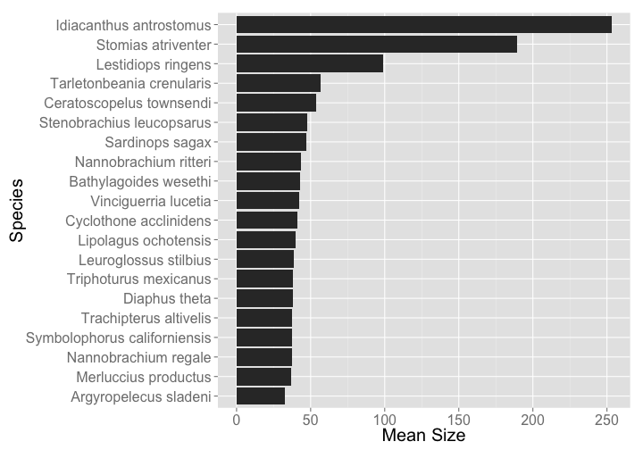
Since both griddap() and tabledap() give back data.frame’s, it’s easy to do downstream manipulation. For example, we can use dplyr to filter, summarize, group, and sort:
library("dplyr")
dat$fish_size <- as.numeric(dat$fish_size)
df <- tbl_df(dat) %>%
  filter(fish_size > 30) %>%
  group_by(scientific_name) %>%
  summarise(mean_size = mean(fish_size)) %>%
  arrange(desc(mean_size))
df
#> Source: local data frame [20 x 2]
#>
#>                 scientific_name mean_size
#> 1       Idiacanthus antrostomus 253.00000
#> 2            Stomias atriventer 189.25000
#> 3            Lestidiops ringens  98.70000
#> 4     Tarletonbeania crenularis  56.50000
#> 5      Ceratoscopelus townsendi  53.70000
#> 6     Stenobrachius leucopsarus  47.74538
#> 7               Sardinops sagax  47.00000
#> 8         Nannobrachium ritteri  43.30250
#> 9         Bathylagoides wesethi  43.09167
#> 10         Vinciguerria lucetia  42.00000
#> 11       Cyclothone acclinidens  40.80000
#> 12         Lipolagus ochotensis  39.72500
#> 13        Leuroglossus stilbius  38.35385
#> 14        Triphoturus mexicanus  38.21342
#> 15                Diaphus theta  37.88571
#> 16       Trachipterus altivelis  37.70000
#> 17 Symbolophorus californiensis  37.66000
#> 18         Nannobrachium regale  37.50000
#> 19         Merluccius productus  36.61333
#> 20        Argyropelecus sladeni  32.43333
Then make a cute little plot
library("ggplot2")
ggplot(df, aes(reorder(scientific_name, mean_size), mean_size)) +
  geom_bar(stat = "identity") +
  coord_flip() +
  theme_grey(base_size = 20) +
  labs(y = "Mean Size", x = "Species")