NOAA provides a lot of weather data, across many different websites under different project names. The R package rnoaa accesses many of these, including:
- NOAA NCDC climate data, using the NCDC API version 2
- GHCND FTP data
- ISD FTP data
- Severe weather data docs are at https://www.ncdc.noaa.gov/swdiws/
- Sea ice data
- NOAA buoy data
- Tornadoes! Data from the NOAA Storm Prediction Center
- HOMR - Historical Observing Metadata Repository - from NOAA NCDC
- Storm data - from the International Best Track Archive for Climate Stewardship (IBTrACS)
rnoaa used to provide access to ERDDAP servers, but a separate package rerddap focuses on just those data sources.
We focus on getting you the data, so there’s very little in rnoaa for visualizing, statistics, etc.
Installation
The newest version should be on CRAN in the next few days. In the meantime, let’s install from GitHub
devtools::install_github("ropensci/rnoaa")
library("rnoaa")
There’s an example using the lawn, sp, and dplyr packages. If you want to try those, install like
install.packages(c("lawn", "dplyr", "sp"))
NCDC
- NCDC = National Climatic Data Center
- Data comes from a RESTful API described at https://www.ncdc.noaa.gov/cdo-web/webservices/v2
This web service requires an API key - get one at https://www.ncdc.noaa.gov/cdo-web/token if you don’t already have one. NCDC provides access to many different datasets:
| Dataset | Description | Start date | End date |
|---|---|---|---|
| ANNUAL | Annual Summaries | 1831-02-01 | 2013-11-01 |
| GHCND | Daily Summaries | 1763-01-01 | 2014-03-15 |
| GHCNDMS | Monthly Summaries | 1763-01-01 | 2014-01-01 |
| NORMAL_ANN | Normals Annual/Seasonal | 2010-01-01 | 2010-01-01 |
| NORMAL_DLY | Normals Daily | 2010-01-01 | 2010-12-31 |
| NORMAL_HLY | Normals Hourly | 2010-01-01 | 2010-12-31 |
| NORMAL_MLY | Normals Monthly | 2010-01-01 | 2010-12-01 |
| PRECIP_15 | Precipitation 15 Minute | 1970-05-12 | 2013-03-01 |
| PRECIP_HLY | Precipitation Hourly | 1900-01-01 | 2013-03-01 |
| NEXRAD2 | Nexrad Level II | 1991-06-05 | 2014-03-14 |
| NEXRAD3 | Nexrad Level III | 1994-05-20 | 2014-03-11 |
The main function to get data from NCDC is ncdc(). datasetid, startdate, and enddate are required parameters. A quick example, here getting data from the GHCND dataset, from a particular station, and from Oct 1st 2013 to Dec 12th 2013:
ncdc(datasetid = 'GHCND', stationid = 'GHCND:USW00014895', startdate = '2013-10-01',
   enddate = '2013-12-01')
#> $meta
#> $meta$totalCount
#> [1] 697
#>
#> $meta$pageCount
#> [1] 25
#>
#> $meta$offset
#> [1] 1
#>
#>
#> $data
#> Source: local data frame [25 x 8]
#>
#>                   date datatype           station value fl_m fl_q fl_so
#> 1  2013-10-01T00:00:00     AWND GHCND:USW00014895    29               W
#> 2  2013-10-01T00:00:00     PRCP GHCND:USW00014895     0               W
#> 3  2013-10-01T00:00:00     SNOW GHCND:USW00014895     0               W
#> 4  2013-10-01T00:00:00     SNWD GHCND:USW00014895     0               W
#> 5  2013-10-01T00:00:00     TAVG GHCND:USW00014895   179    H          S
#> 6  2013-10-01T00:00:00     TMAX GHCND:USW00014895   250               W
#> 7  2013-10-01T00:00:00     TMIN GHCND:USW00014895   133               W
#> 8  2013-10-01T00:00:00     WDF2 GHCND:USW00014895   210               W
#> 9  2013-10-01T00:00:00     WDF5 GHCND:USW00014895   230               W
#> 10 2013-10-01T00:00:00     WSF2 GHCND:USW00014895    76               W
#> ..                 ...      ...               ...   ...  ...  ...   ...
#> Variables not shown: fl_t (chr)
#>
#> attr(,"class")
#> [1] "ncdc_data"
You probably won’t know what station you want data from off hand though, so you can first search for stations, in this example using a bounding box that defines a rectangular area near Seattle
library("lawn")
lawn_bbox_polygon(c(-122.2047, 47.5204, -122.1065, 47.6139)) %>% view
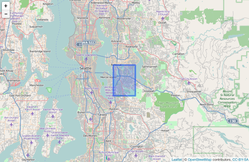
We’ll search within that bounding box for weather stations.
ncdc_stations(extent = c(47.5204, -122.2047, 47.6139, -122.1065))
#> $meta
#> $meta$totalCount
#> [1] 9
#>
#> $meta$pageCount
#> [1] 25
#>
#> $meta$offset
#> [1] 1
#>
#>
#> $data
#> Source: local data frame [9 x 9]
#>
#>   elevation    mindate    maxdate latitude                         name
#> 1     199.6 2008-06-01 2015-06-29  47.5503      EASTGATE 1.7 SSW, WA US
#> 2     240.8 2010-05-01 2015-07-05  47.5604       EASTGATE 1.1 SW, WA US
#> 3      85.6 2008-07-01 2015-07-05  47.5916        BELLEVUE 0.8 S, WA US
#> 4     104.2 2008-06-01 2015-07-05  47.5211 NEWPORT HILLS 1.9 SSE, WA US
#> 5      58.5 2008-08-01 2009-04-12  47.6138      BELLEVUE 2.3 ENE, WA US
#> 6     199.9 2008-06-01 2009-11-22  47.5465   NEWPORT HILLS 1.4 E, WA US
#> 7      27.1 2008-07-01 2015-07-05  47.6046        BELLEVUE 1.8 W, WA US
#> 8     159.4 2008-11-01 2015-07-05  47.5694      BELLEVUE 2.3 SSE, WA US
#> 9      82.3 2008-12-01 2010-09-17  47.6095       BELLEVUE 0.6 NE, WA US
#> Variables not shown: datacoverage (dbl), id (chr), elevationUnit (chr),
#>   longitude (dbl)
#>
#> attr(,"class")
#> [1] "ncdc_stations"
And there are 9 found. We could then use their station ids (e.g., GHCND:US1WAKG0024) to search for data using ncdc(), or search for what kind of data that station has with ncdc_datasets(), or other functions.
GHCND
- GHCND = Global Historical Climatology Network Daily (Data)
- Data comes from an FTP server
library("dplyr")
dat <- ghcnd(stationid = "AGE00147704")
dat$data %>%
  filter(element == "PRCP", year == 1909)
#>            id year month element VALUE1 MFLAG1 QFLAG1 SFLAG1 VALUE2 MFLAG2
#> 1 AGE00147704 1909    11    PRCP  -9999     NA                -9999     NA
#> 2 AGE00147704 1909    12    PRCP     23     NA             E      0     NA
#>   QFLAG2 SFLAG2 VALUE3 MFLAG3 QFLAG3 SFLAG3 VALUE4 MFLAG4 QFLAG4 SFLAG4
#> 1                -9999     NA                -9999     NA
#> 2             E      0     NA             E      0     NA             E
#>   VALUE5 MFLAG5 QFLAG5 SFLAG5 VALUE6 MFLAG6 QFLAG6 SFLAG6 VALUE7 MFLAG7
#> 1  -9999     NA                -9999     NA                -9999     NA
#> 2      0     NA             E      0     NA             E      0     NA
#>   QFLAG7 SFLAG7 VALUE8 MFLAG8 QFLAG8 SFLAG8 VALUE9 MFLAG9 QFLAG9 SFLAG9
#> 1     NA         -9999     NA                -9999     NA
#> 2     NA      E    250     NA             E     75     NA             E
#>   VALUE10 MFLAG10 QFLAG10 SFLAG10 VALUE11 MFLAG11 QFLAG11 SFLAG11 VALUE12
#> 1   -9999      NA                   -9999      NA                   -9999
#> 2     131      NA               E       0      NA               E       0
#>   MFLAG12 QFLAG12 SFLAG12 VALUE13 MFLAG13 QFLAG13 SFLAG13 VALUE14 MFLAG14
#> 1      NA                   -9999      NA                   -9999      NA
#> 2      NA               E       0      NA               E       0      NA
#>   QFLAG14 SFLAG14 VALUE15 MFLAG15 QFLAG15 SFLAG15 VALUE16 MFLAG16 QFLAG16
#> 1                   -9999      NA                   -9999      NA
#> 2               E       0      NA               E       0      NA
#>   SFLAG16 VALUE17 MFLAG17 QFLAG17 SFLAG17 VALUE18 MFLAG18 QFLAG18 SFLAG18
#> 1           -9999      NA                   -9999      NA
#> 2       E       0      NA               E       0      NA               E
#>   VALUE19 MFLAG19 QFLAG19 SFLAG19 VALUE20 MFLAG20 QFLAG20 SFLAG20 VALUE21
#> 1   -9999      NA      NA           -9999      NA      NA           -9999
#> 2       0      NA      NA       E       0      NA      NA       E       0
#>   MFLAG21 QFLAG21 SFLAG21 VALUE22 MFLAG22 QFLAG22 SFLAG22 VALUE23 MFLAG23
#> 1      NA                   -9999      NA                      22      NA
#> 2      NA               E       0      NA               E       0      NA
#>   QFLAG23 SFLAG23 VALUE24 MFLAG24 QFLAG24 SFLAG24 VALUE25 MFLAG25 QFLAG25
#> 1      NA       E       9      NA      NA       E       5      NA      NA
#> 2      NA       E       0      NA      NA       E       0      NA      NA
#>   SFLAG25 VALUE26 MFLAG26 QFLAG26 SFLAG26 VALUE27 MFLAG27 QFLAG27 SFLAG27
#> 1       E       0      NA               E      86      NA      NA       E
#> 2       E       0      NA               E       0      NA      NA       E
#>   VALUE28 MFLAG28 QFLAG28 SFLAG28 VALUE29 MFLAG29 QFLAG29 SFLAG29 VALUE30
#> 1       0      NA      NA       E      28      NA      NA       E       0
#> 2       0      NA      NA       E       0      NA      NA       E       0
#>   MFLAG30 QFLAG30 SFLAG30 VALUE31 MFLAG31 QFLAG31 SFLAG31
#> 1      NA               E   -9999      NA      NA
#> 2      NA               E      57      NA      NA       E
You can also get to datasets by searching by station id, date min, date max, and variable. E.g.
ghcnd_search("AGE00147704", var = "PRCP")
#> $prcp
#> Source: local data frame [9,803 x 6]
#>
#>             id  prcp       date mflag qflag sflag
#> 1  AGE00147704 -9999 1909-11-01    NA
#> 2  AGE00147704    23 1909-12-01    NA           E
#> 3  AGE00147704    81 1910-01-01    NA           E
#> 4  AGE00147704     0 1910-02-01    NA           E
#> 5  AGE00147704    18 1910-03-01    NA           E
#> 6  AGE00147704     0 1910-04-01    NA           E
#> 7  AGE00147704   223 1910-05-01    NA           E
#> 8  AGE00147704     0 1910-06-01    NA           E
#> 9  AGE00147704     0 1910-07-01    NA           E
#> 10 AGE00147704     0 1910-08-01    NA           E
#> ..         ...   ...        ...   ...   ...   ...
ISD
- ISD = Integrated Surface Database
- Data comes from an FTP server
You’ll likely first want to run isd_stations() to get list of stations
stations <- isd_stations()
head(stations)
#>   usaf  wban station_name ctry state icao lat lon elev_m    begin      end
#> 1 7005 99999   CWOS 07005                  NA  NA     NA 20120127 20120127
#> 2 7011 99999   CWOS 07011                  NA  NA     NA 20111025 20121129
#> 3 7018 99999   WXPOD 7018                   0   0   7018 20110309 20130730
#> 4 7025 99999   CWOS 07025                  NA  NA     NA 20120127 20120127
#> 5 7026 99999   WXPOD 7026   AF              0   0   7026 20120713 20141120
#> 6 7034 99999   CWOS 07034                  NA  NA     NA 20121024 20121106
Then get data from particular stations, like
(res <- isd(usaf = "011490", wban = "99999", year = 1986))
#> <ISD Data>
#> Size: 1328 X 85
#>
#>    total_chars usaf_station wban_station     date time date_flag latitude
#> 1           50        11490        99999 19860101    0         4    66267
#> 2          123        11490        99999 19860101  600         4    66267
#> 3           50        11490        99999 19860101 1200         4    66267
#> 4           94        11490        99999 19860101 1800         4    66267
#> 5           50        11490        99999 19860102    0         4    66267
#> 6          123        11490        99999 19860102  600         4    66267
#> 7           50        11490        99999 19860102 1200         4    66267
#> 8           94        11490        99999 19860102 1800         4    66267
#> 9           50        11490        99999 19860103    0         4    66267
#> 10         123        11490        99999 19860103  600         4    66267
#> ..         ...          ...          ...      ...  ...       ...      ...
#> Variables not shown: longitude (int), type_code (chr), elevation (int),
#>      call_letter (int), quality (chr), wind_direction (int),
#>      wind_direction_quality (int), wind_code (chr), wind_speed (int),
#>      wind_speed_quality (int), ceiling_height (int),
#>      ceiling_height_quality (int), ceiling_height_determination (chr),
#>      ceiling_height_cavok (chr), visibility_distance (int),
#>      visibility_distance_quality (int), visibility_code (chr),
#>      visibility_code_quality (int), temperature (int), temperature_quality
#>      (int), temperature_dewpoint (int), temperature_dewpoint_quality
#>      (int), air_pressure (int), air_pressure_quality (int),
#>      AG1.precipitation (chr), AG1.discrepancy (int), AG1.est_water_depth
#>      (int), GF1.sky_condition (chr), GF1.coverage (int),
#>      GF1.opaque_coverage (int), GF1.coverage_quality (int),
#>      GF1.lowest_cover (int), GF1.lowest_cover_quality (int),
#>      GF1.low_cloud_genus (int), GF1.low_cloud_genus_quality (int),
#>      GF1.lowest_cloud_base_height (int),
#>      GF1.lowest_cloud_base_height_quality (int), GF1.mid_cloud_genus
#>      (int), GF1.mid_cloud_genus_quality (int), GF1.high_cloud_genus (int),
#>      GF1.high_cloud_genus_quality (int), MD1.atmospheric_change (chr),
#>      MD1.tendency (int), MD1.tendency_quality (int), MD1.three_hr (int),
#>      MD1.three_hr_quality (int), MD1.twentyfour_hr (int),
#>      MD1.twentyfour_hr_quality (int), REM.remarks (chr), REM.identifier
#>      (chr), REM.length_quantity (int), REM.comment (chr), KA1.extreme_temp
#>      (chr), KA1.period_quantity (int), KA1.max_min (chr), KA1.temp (int),
#>      KA1.temp_quality (int), AY1.manual_occurrence (chr),
#>      AY1.condition_code (int), AY1.condition_quality (int), AY1.period
#>      (int), AY1.period_quality (int), AY2.manual_occurrence (chr),
#>      AY2.condition_code (int), AY2.condition_quality (int), AY2.period
#>      (int), AY2.period_quality (int), MW1.first_weather_reported (chr),
#>      MW1.condition (int), MW1.condition_quality (int),
#>      EQD.observation_identifier (chr), EQD.observation_text (int),
#>      EQD.reason_code (int), EQD.parameter (chr),
#>      EQD.observation_identifier.1 (chr), EQD.observation_text.1 (int),
#>      EQD.reason_code.1 (int), EQD.parameter.1 (chr)
Severe weather
- SWDI = Severe Weather Data Inventory
- From the SWDI site
The Severe Weather Data Inventory (SWDI) is an integrated database of severe weather records for the United States. The records in SWDI come from a variety of sources in the NCDC archive.
The swdi() function allows you to get data in xml, csv, shp, or kmz format. You can get data from many different datasets:
- nx3tvs NEXRAD Level-3 Tornado Vortex Signatures (point)
- nx3meso NEXRAD Level-3 Mesocyclone Signatures (point)
- nx3hail NEXRAD Level-3 Hail Signatures (point)
- nx3structure NEXRAD Level-3 Storm Cell Structure Information (point)
- plsr Preliminary Local Storm Reports (point)
- warn Severe Thunderstorm, Tornado, Flash Flood and Special Marine warnings (polygon)
- nldn Lightning strikes from Vaisala (.gov and .mil ONLY) (point)
An example: Get all plsr within the bounding box (-91,30,-90,31)
swdi(dataset = 'plsr', startdate = '20060505', enddate = '20060510',
bbox = c(-91, 30, -90, 31))
#> $meta
#> $meta$totalCount
#> numeric(0)
#>
#> $meta$totalTimeInSeconds
#> [1] 0
#>
#>
#> $data
#> Source: local data frame [5 x 8]
#>
#>                  ztime     id        event magnitude            city
#> 1 2006-05-09T02:20:00Z 427540         HAIL         1    5 E KENTWOOD
#> 2 2006-05-09T02:40:00Z 427536         HAIL         1    MOUNT HERMAN
#> 3 2006-05-09T02:40:00Z 427537 TSTM WND DMG     -9999    MOUNT HERMAN
#> 4 2006-05-09T03:00:00Z 427199         HAIL         0     FRANKLINTON
#> 5 2006-05-09T03:17:00Z 427200      TORNADO     -9999 5 S FRANKLINTON
#> Variables not shown: county (chr), state (chr), source (chr)
#>
#> $shape
#>                  shape
#> 1 POINT (-90.43 30.93)
#> 2  POINT (-90.3 30.96)
#> 3  POINT (-90.3 30.96)
#> 4 POINT (-90.14 30.85)
#> 5 POINT (-90.14 30.78)
#>
#> attr(,"class")
#> [1] "swdi"
Sea ice
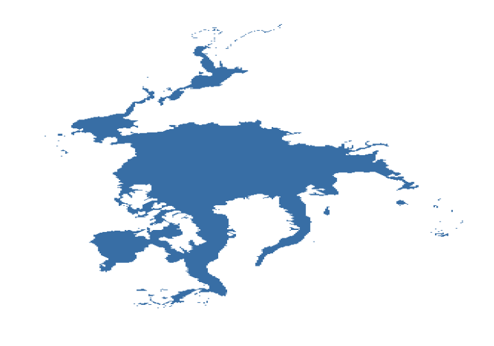
The seaice() function simply grabs shape files that describe sea ice cover at the Northa and South poles, and can be useful for examining change through time in sea ice cover, among other things.
An example: Plot sea ice cover for April 1990 for the North pole.
urls <- seaiceeurls(mo = 'Apr', pole = 'N', yr = 1990)
out <- seaice(urls)

library('ggplot2')
ggplot(out, aes(long, lat, group = group)) +
   geom_polygon(fill = "steelblue") +
   theme_ice()
Buoys
- Get NOAA buoy data from the National Buoy Data Center
Using buoy data requires the ncdf package. Make sure you have that installed, like install.packages("ncdf"). buoy() and buoys() will fail if you don’t have ncdf installed.
buoys() - Get available buoys given a dataset name
head(buoys(dataset = 'cwind'))
#>      id
#> 1 41001
#> 2 41002
#> 3 41004
#> 4 41006
#> 5 41008
#> 6 41009
#>                                                                       url
#> 1 https://dods.ndbc.noaa.gov/thredds/catalog/data/cwind/41001/catalog.html
#> 2 https://dods.ndbc.noaa.gov/thredds/catalog/data/cwind/41002/catalog.html
#> 3 https://dods.ndbc.noaa.gov/thredds/catalog/data/cwind/41004/catalog.html
#> 4 https://dods.ndbc.noaa.gov/thredds/catalog/data/cwind/41006/catalog.html
#> 5 https://dods.ndbc.noaa.gov/thredds/catalog/data/cwind/41008/catalog.html
#> 6 https://dods.ndbc.noaa.gov/thredds/catalog/data/cwind/41009/catalog.html
buoy() - Get data for a buoy - if no year or datatype specified, we get the first file
buoy(dataset = 'cwind', buoyid = 46085)
#> Dimensions (rows/cols): [33486 X 5]
#> 2 variables: [wind_dir, wind_spd]
#>
#>                    time latitude longitude wind_dir wind_spd
#> 1  2007-05-05T02:00:00Z   55.855  -142.559      331      2.8
#> 2  2007-05-05T02:10:00Z   55.855  -142.559      328      2.6
#> 3  2007-05-05T02:20:00Z   55.855  -142.559      329      2.2
#> 4  2007-05-05T02:30:00Z   55.855  -142.559      356      2.1
#> 5  2007-05-05T02:40:00Z   55.855  -142.559      360      1.5
#> 6  2007-05-05T02:50:00Z   55.855  -142.559       10      1.9
#> 7  2007-05-05T03:00:00Z   55.855  -142.559       10      2.2
#> 8  2007-05-05T03:10:00Z   55.855  -142.559       14      2.2
#> 9  2007-05-05T03:20:00Z   55.855  -142.559       16      2.1
#> 10 2007-05-05T03:30:00Z   55.855  -142.559       22      1.6
#> ..                  ...      ...       ...      ...      ...
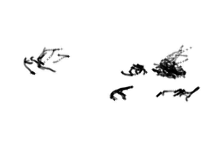
Tornadoes
The function tornadoes() gets tornado data from https://www.spc.noaa.gov/gis/svrgis/.
shp <- tornadoes()
library('sp')
plot(shp)

Historical Observing Metadata Repository
- HOMR = Historical Observing Metadata Repository
- Data from RESTful API at https://www.ncdc.noaa.gov/homr/api
homr_definitions() gets you definitions and metadata for datasets
head(homr_definitions())
#> Source: local data frame [6 x 7]
#>
#>   defType  abbr                fullName    displayName
#> 1     ids GHCND        GHCND IDENTIFIER       GHCND ID
#> 2     ids  COOP             COOP NUMBER        COOP ID
#> 3     ids  WBAN             WBAN NUMBER        WBAN ID
#> 4     ids   FAA FAA LOCATION IDENTIFIER         FAA ID
#> 5     ids  ICAO                 ICAO ID        ICAO ID
#> 6     ids TRANS          TRANSMITTAL ID Transmittal ID
#> Variables not shown: description (chr), cssaName (chr), ghcndName (chr)
homr() gets you metadata for stations given query parameters. In this example, search for data for the state of Delaware
res <- homr(state = 'DE')
names(res) # the stations
#>  [1] "10001871" "10100162" "10100164" "10100166" "20004155" "20004158"
#>  [7] "20004160" "20004162" "20004163" "20004168" "20004171" "20004176"
#> [13] "20004178" "20004179" "20004180" "20004182" "20004184" "20004185"
#> [19] "30001831" "30017384" "30020917" "30021161" "30021998" "30022674"
#> [25] "30026770" "30027455" "30032423" "30032685" "30034222" "30039554"
#> [31] "30043742" "30046662" "30046814" "30051475" "30057217" "30063570"
#> [37] "30064900" "30065901" "30067636" "30069663" "30075067" "30077378"
#> [43] "30077857" "30077923" "30077988" "30079088" "30079240" "30082430"
#> [49] "30084216" "30084262" "30084537" "30084796" "30094582" "30094639"
#> [55] "30094664" "30094670" "30094683" "30094730" "30094806" "30094830"
#> [61] "30094917" "30094931" "30094936" "30094991"
You can index to each one to get more data
Storms
- Data from: International Best Track Archive for Climate Stewardship (IBTrACS)
- Data comes from an FTP server
Flat files (csv’s) are served up as well as shp files. In this example, plot storm data for the year 1940
(res3 <- storm_shp(year = 1940))
#> <NOAA Storm Shp Files>
#> Path: ~/.rnoaa/storms/year/Year.1940.ibtracs_all_points.v03r06.shp
#> Basin: <NA>
#> Storm: <NA>
#> Year: 1940
#> Type: points
res3shp <- storm_shp_read(res3)
sp::plot(res3shp)