Finally, we got fulltext up on CRAN - our first commit was May last year. fulltext is a package to facilitate text mining. It focuses on open access journals. This package makes it easier to search for articles, download those articles in full text if available, convert pdf format to plain text, and extract text chunks for vizualization/analysis. We are planning to add bits for analysis in future versions. We’ve been working on this package for a while now. It has a lot of moving parts and package dependencies, so it took a while to get a first useable version.
The tasks facilitated by fulltext in bullet form:
- Search - search for articles
- Retrieve - get full text
- Convert - convert from format X to Y
- Text - if needed, get text from pdfs/etc.
- Extract - pull out the bits of articles that you want
I won’t be surprised if users uncover a lot of bugs in this package given the huge number of publishers/journals users want to get literature data from, and the surely wide diversity of use cases. But I thought it was important to get out a first version to get feedback on the user interface, and gather use cases.
We hope that this package can help bring text-mining to the masses - making it easy for anyone to do do, not just text-mining experts.
If you have any feedback, please do get in touch in the issue tracker for fulltext at https://github.com/ropensci/fulltext/issues - If you have use case thoughts, the rOpenSci discussion forum might be a good place to go.
Let’s kick the tires, shall we?
Install
Will be on CRAN soon, not as of AM PDT on 2015-08-07.
install.packages("fulltext")
# if binaries not avail. yet on your favorite CRAN mirror
install.packages("https://cran.rstudio.com/src/contrib/fulltext_0.1.0.tar.gz", repos = NULL, type = "source")
Or install development version from GitHub
devtools::install_github("ropensci/fulltext")
Load fulltext
library("fulltext")
Search for articles
Currently, there are hooks for searching for articles from PLOS, BMC, Crossref, Entrez, arXiv, and BioRxiv. We’ll add more in the future, but that does cover a lot of articles, especially given inclusion of Crossref (which mints most DOIs) and Entrez (which houses PMC and Pubmed).
An example: Search for the term ecology in PLOS journals.
(res1 <- ft_search(query = 'ecology', from = 'plos'))
#> Query:
#>   [ecology]
#> Found:
#>   [PLoS: 28589; BMC: 0; Crossref: 0; Entrez: 0; arxiv: 0; biorxiv: 0]
#> Returned:
#>   [PLoS: 10; BMC: 0; Crossref: 0; Entrez: 0; arxiv: 0; biorxiv: 0]
Each publisher/search-engine has a slot with metadata and data, saying how many articles were found and how many were returned. We can dig into what PLOS gave us:
res1$plos
#> Query: [ecology]
#> Records found, returned: [28589, 10]
#> License: [CC-BY]
#>                                                         id
#> 1                             10.1371/journal.pone.0059813
#> 2                             10.1371/journal.pone.0001248
#> 3  10.1371/annotation/69333ae7-757a-4651-831c-f28c5eb02120
#> 4                             10.1371/journal.pone.0080763
#> 5                             10.1371/journal.pone.0102437
#> 6                             10.1371/journal.pone.0017342
#> 7                             10.1371/journal.pone.0091497
#> 8                             10.1371/journal.pone.0092931
#> 9  10.1371/annotation/28ac6052-4f87-4b88-a817-0cd5743e83d6
#> 10                            10.1371/journal.pcbi.1003594
For each of the data sources to search on you can pass in additional options (basically, you can use the query parameters in the functions that hit each service). Here, we can modify our search to PLOS by requesting a particular set of fields with the fl parameter (PLOS uses a Solr backed search engine, and fl is short for fields in Solr land):
ft_search(query = 'ecology', from = 'plos', plosopts = list(
   fl = c('id','author','eissn','journal','counter_total_all','alm_twitterCount')))
#> Query:
#>   [ecology]
#> Found:
#>   [PLoS: 28589; BMC: 0; Crossref: 0; Entrez: 0; arxiv: 0; biorxiv: 0]
#> Returned:
#>   [PLoS: 10; BMC: 0; Crossref: 0; Entrez: 0; arxiv: 0; biorxiv: 0]
Note that PLOS is a bit unique in allowing you to request specific parts of articles. Other sources in ft_search() don’t let you do that.
Get full text
After you’ve found the set of articles you want to get full text for, we can use the results from ft_search() to grab full text. ft_get() accepts a character vector of list of DOIs (or PMC IDs if fetching from Entrez), or the output of ft_search().
(out <- ft_get(res1))
#> [Docs] 8
#> [Source] R session
#> [IDs] 10.1371/journal.pone.0059813 10.1371/journal.pone.0001248
#>      10.1371/journal.pone.0080763 10.1371/journal.pone.0102437
#>      10.1371/journal.pone.0017342 10.1371/journal.pone.0091497
#>      10.1371/journal.pone.0092931 10.1371/journal.pcbi.1003594 ...
We got eight articles in full text in the result. We didn’t get 10, even though 10 were returned from ft_search() because PLOS often returns records for annotations, that is, comments on articles, which we auto-seive out within ft_get().
Dig in to the PLOS data
out$plos
#> $found
#> [1] 8
#>
#> $dois
#> [1] "10.1371/journal.pone.0059813" "10.1371/journal.pone.0001248"
#> [3] "10.1371/journal.pone.0080763" "10.1371/journal.pone.0102437"
#> [5] "10.1371/journal.pone.0017342" "10.1371/journal.pone.0091497"
#> [7] "10.1371/journal.pone.0092931" "10.1371/journal.pcbi.1003594"
#>
#> $data
#> $data$backend
#> NULL
#>
#> $data$path
#> [1] "session"
#>
#> $data$data
#> 8 full-text articles retrieved
#> Min. Length: 3828 - Max. Length: 104702
#> DOIs: 10.1371/journal.pone.0059813 10.1371/journal.pone.0001248
#>   10.1371/journal.pone.0080763 10.1371/journal.pone.0102437
#>   10.1371/journal.pone.0017342 10.1371/journal.pone.0091497
#>   10.1371/journal.pone.0092931 10.1371/journal.pcbi.1003594 ...
#>
#> NOTE: extract xml strings like output['<doi>']
#>
#> $opts
#> $opts$doi
#> [1] "10.1371/journal.pone.0059813" "10.1371/journal.pone.0001248"
#> [3] "10.1371/journal.pone.0080763" "10.1371/journal.pone.0102437"
#> [5] "10.1371/journal.pone.0017342" "10.1371/journal.pone.0091497"
#> [7] "10.1371/journal.pone.0092931" "10.1371/journal.pcbi.1003594"
#>
#> $opts$callopts
#> list()
Dig in further to get to one of the articles in XML format
library("xml2")
xml2::read_xml(out$plos$data$data$`10.1371/journal.pone.0059813`)
#> {xml_document}
#> <article>
#> [1] <front>\n<journal-meta>\n<journal-id journal-id-type="nlm-ta">PLoS O ...
#> [2] <body>\n  <sec id="s1">\n<title>Introduction</title>\n<p>Ecologists  ...
#> [3] <back>\n<ack>\n<p>Curtis Flather, Mark Burgman, Leon Blaustein, Yaac ...
Now with the xml, you can dig into whatever you like, e.g., using xml2 or rvest.
Extract text from pdfs
Ideally for text mining you have access to XML or other text based formats. However, sometimes you only have access to PDFs. In this case you want to extract text from PDFs. fulltext can help with that.
You can extract from any pdf from a file path, like:
path <- system.file("examples", "example1.pdf", package = "fulltext")
ft_extract(path)
#> <document>/Library/Frameworks/R.framework/Versions/3.2/Resources/library/fulltext/examples/example1.pdf
#>   Pages: 18
#>   Title: Suffering and mental health among older people living in nursing homes---a mixed-methods study
#>   Producer: pdfTeX-1.40.10
#>   Creation date: 2015-07-17
Let’s search for articles from arXiv, a preprint service. Here, get pdf from an article with ID cond-mat/9309029:
res <- ft_get('cond-mat/9309029', from = "arxiv")
res2 <- ft_extract(res)
res2$arxiv$data
#> $backend
#> NULL
#>
#> $path
#> $path$`cond-mat/9309029`
#> [1] "~/.fulltext/cond-mat_9309029.pdf"
#>
#>
#> $data
#> $data[[1]]
#> <document>/Users/sacmac/.fulltext/cond-mat_9309029.pdf
#>   Pages: 14
#>   Title: arXiv:cond-mat/9309029v8  26 Jan 1994
#>   Producer: GPL Ghostscript SVN PRE-RELEASE 8.62
#>   Creation date: 2008-02-06
And a short snippet of the full text
res2$arxiv$data$data[[1]]$data
#> "arXiv:cond-mat/9309029v8 26 Jan 1994, , FERMILAB-PUB-93/15-T March 1993, Revised:
#> January 1994, The Thermodynamics and Economics of Waste, Dallas C. Kennedy, Research
#> Associate, Fermi National Accelerator Laboratory, P.O. Box 500 MS106, Batavia, Illinois
#> 60510 USA, Abstract, The increasingly relevant problem of natural resource use and
#> waste production, disposal, and reuse is examined from several viewpoints: economic,
#> technical, and thermodynamic. Alternative economies are studied, with emphasis on
#> recycling of waste to close the natural resource cycle. The physical nature of human
#> economies and constraints on recycling and energy efficiency are stated in terms
#> ..."
Extract text chunks
We have a few functions to help you pull out certain parts of an article. For example, perhaps you want to get just the authors from your articles, or just the abstracts.
Here, we’ll search for some PLOS articles, then get their full text, then extract various parts of each article with chunks().
res <- ft_search(query = "ecology", from = "plos")
(x <- ft_get(res))
#> [Docs] 8
#> [Source] R session
#> [IDs] 10.1371/journal.pone.0059813 10.1371/journal.pone.0001248
#>      10.1371/journal.pone.0080763 10.1371/journal.pone.0102437
#>      10.1371/journal.pone.0017342 10.1371/journal.pone.0091497
#>      10.1371/journal.pone.0092931 10.1371/journal.pcbi.1003594 ...
Extract DOIs
x %>% chunks("doi")
#> $plos
#> $plos$`10.1371/journal.pone.0059813`
#> $plos$`10.1371/journal.pone.0059813`$doi
#> [1] "10.1371/journal.pone.0059813"
#>
#>
#> $plos$`10.1371/journal.pone.0001248`
#> $plos$`10.1371/journal.pone.0001248`$doi
#> [1] "10.1371/journal.pone.0001248"
#>
#>
#> $plos$`10.1371/journal.pone.0080763`
#> $plos$`10.1371/journal.pone.0080763`$doi
#> [1] "10.1371/journal.pone.0080763"
#>
#>
#> $plos$`10.1371/journal.pone.0102437`
#> $plos$`10.1371/journal.pone.0102437`$doi
#> [1] "10.1371/journal.pone.0102437"
#>
#>
#> $plos$`10.1371/journal.pone.0017342`
#> $plos$`10.1371/journal.pone.0017342`$doi
#> [1] "10.1371/journal.pone.0017342"
#>
#>
#> $plos$`10.1371/journal.pone.0091497`
#> $plos$`10.1371/journal.pone.0091497`$doi
#> [1] "10.1371/journal.pone.0091497"
#>
#>
#> $plos$`10.1371/journal.pone.0092931`
#> $plos$`10.1371/journal.pone.0092931`$doi
#> [1] "10.1371/journal.pone.0092931"
#>
#>
#> $plos$`10.1371/journal.pcbi.1003594`
#> $plos$`10.1371/journal.pcbi.1003594`$doi
#> [1] "10.1371/journal.pcbi.1003594"
Extract DOIs and categories
x %>% chunks(c("doi","categories"))
#> $plos
#> $plos$`10.1371/journal.pone.0059813`
#> $plos$`10.1371/journal.pone.0059813`$doi
#> [1] "10.1371/journal.pone.0059813"
#>
#> $plos$`10.1371/journal.pone.0059813`$categories
#>  [1] "Research Article"                 "Biology"
#>  [3] "Ecology"                          "Community ecology"
#>  [5] "Species interactions"             "Science policy"
#>  [7] "Research assessment"              "Research monitoring"
#>  [9] "Research funding"                 "Government funding of science"
#> [11] "Research laboratories"            "Science policy and economics"
#> [13] "Science and technology workforce" "Careers in research"
#> [15] "Social and behavioral sciences"   "Sociology"
#> [17] "Sociology of knowledge"
#>
#>
#> $plos$`10.1371/journal.pone.0001248`
#> $plos$`10.1371/journal.pone.0001248`$doi
#> [1] "10.1371/journal.pone.0001248"
#>
#> $plos$`10.1371/journal.pone.0001248`$categories
#> [1] "Research Article"             "Ecology"
#> [3] "Ecology/Ecosystem Ecology"    "Ecology/Evolutionary Ecology"
#> [5] "Ecology/Theoretical Ecology"
#>
#>
#> $plos$`10.1371/journal.pone.0080763`
#> $plos$`10.1371/journal.pone.0080763`$doi
#> [1] "10.1371/journal.pone.0080763"
#>
#> $plos$`10.1371/journal.pone.0080763`$categories
#>  [1] "Research Article"     "Biology"              "Ecology"
#>  [4] "Autecology"           "Behavioral ecology"   "Community ecology"
#>  [7] "Evolutionary ecology" "Population ecology"   "Evolutionary biology"
#> [10] "Behavioral ecology"   "Evolutionary ecology" "Population biology"
#> [13] "Population ecology"
#>
#>
#> $plos$`10.1371/journal.pone.0102437`
#> $plos$`10.1371/journal.pone.0102437`$doi
#> [1] "10.1371/journal.pone.0102437"
#>
#> $plos$`10.1371/journal.pone.0102437`$categories
#>  [1] "Research Article"
#>  [2] "Biology and life sciences"
#>  [3] "Biogeography"
#>  [4] "Ecology"
#>  [5] "Ecosystems"
#>  [6] "Ecosystem engineering"
#>  [7] "Ecosystem functioning"
#>  [8] "Industrial ecology"
#>  [9] "Spatial and landscape ecology"
#> [10] "Urban ecology"
#> [11] "Computer and information sciences"
#> [12] "Geoinformatics"
#> [13] "Spatial analysis"
#> [14] "Earth sciences"
#> [15] "Geography"
#> [16] "Human geography"
#> [17] "Cultural geography"
#> [18] "Social geography"
#> [19] "Ecology and environmental sciences"
#> [20] "Conservation science"
#> [21] "Environmental protection"
#> [22] "Nature-society interactions"
#>
#>
#> $plos$`10.1371/journal.pone.0017342`
#> $plos$`10.1371/journal.pone.0017342`$doi
#> [1] "10.1371/journal.pone.0017342"
#>
#> $plos$`10.1371/journal.pone.0017342`$categories
#>  [1] "Research Article"     "Biology"              "Ecology"
#>  [4] "Community ecology"    "Community assembly"   "Community structure"
#>  [7] "Niche construction"   "Ecological metrics"   "Species diversity"
#> [10] "Species richness"     "Biodiversity"         "Biogeography"
#> [13] "Population ecology"   "Mathematics"          "Statistics"
#> [16] "Biostatistics"        "Statistical theories" "Ecology"
#> [19] "Mathematics"
#>
#>
#> $plos$`10.1371/journal.pone.0091497`
#> $plos$`10.1371/journal.pone.0091497`$doi
#> [1] "10.1371/journal.pone.0091497"
#>
#> $plos$`10.1371/journal.pone.0091497`$categories
#> [1] "Correction"
#>
#>
#> $plos$`10.1371/journal.pone.0092931`
#> $plos$`10.1371/journal.pone.0092931`$doi
#> [1] "10.1371/journal.pone.0092931"
#>
#> $plos$`10.1371/journal.pone.0092931`$categories
#> [1] "Correction"
#>
#>
#> $plos$`10.1371/journal.pcbi.1003594`
#> $plos$`10.1371/journal.pcbi.1003594`$doi
#> [1] "10.1371/journal.pcbi.1003594"
#>
#> $plos$`10.1371/journal.pcbi.1003594`$categories
#> [1] "Research Article"          "Biology and life sciences"
#> [3] "Computational biology"     "Microbiology"
#> [5] "Theoretical biology"
tabularize attempts to help you put the data that comes out of chunks() in to a data.frame, that we all know and love.
x %>% chunks(c("doi", "history")) %>% tabularize()
#> $plos
#>                            doi history.received history.accepted
#> 1 10.1371/journal.pone.0059813       2012-09-16       2013-02-19
#> 2 10.1371/journal.pone.0001248       2007-07-02       2007-11-06
#> 3 10.1371/journal.pone.0080763       2013-08-15       2013-10-16
#> 4 10.1371/journal.pone.0102437       2013-11-27       2014-06-19
#> 5 10.1371/journal.pone.0017342       2010-08-24       2011-01-31
#> 6 10.1371/journal.pone.0091497             <NA>             <NA>
#> 7 10.1371/journal.pone.0092931             <NA>             <NA>
#> 8 10.1371/journal.pcbi.1003594       2014-01-09       2014-03-14
Bring it all together
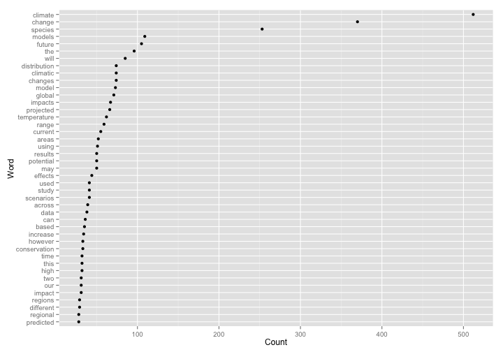
With the pieces above, let’s see what it looks like all in one go. Here, we’ll search for articles on climate change, then visualize word usage in those articles.
Search
(out <- ft_search(query = 'climate change', from = 'plos', limit = 100))
#> Query:
#>   [climate change]
#> Found:
#>   [PLoS: 11737; BMC: 0; Crossref: 0; Entrez: 0; arxiv: 0; biorxiv: 0]
#> Returned:
#>   [PLoS: 100; BMC: 0; Crossref: 0; Entrez: 0; arxiv: 0; biorxiv: 0]
Get full text
(texts <- ft_get(out))
#> [Docs] 99
#> [Source] R session
#> [IDs] 10.1371/journal.pone.0054839 10.1371/journal.pone.0045683
#>      10.1371/journal.pone.0050182 10.1371/journal.pone.0118489
#>      10.1371/journal.pone.0053646 10.1371/journal.pone.0015103
#>      10.1371/journal.pone.0008320 10.1371/journal.pmed.1001227
#>      10.1371/journal.pmed.1001374 10.1371/journal.pone.0097480 ...
Because PLOS returns XML, we don’t need to do a PDF extraction step. However, if we got full text from arXiv or bioRxiv, we’d need to extract from PDFs first.
Pull out chunks
abs <- texts %>% chunks("abstract")
Let’s pull out just the text
abs <- lapply(abs$plos, function(z) {
  paste0(z$abstract, collapse = " ")
})
Analyze
Using the tm package, we can analyze our articles
library("tm")
corp <- VCorpus(VectorSource(abs))
# remove stop words, strip whitespace, remove punctuation
corp <- tm_map(corp, removeWords, stopwords("english"))
corp <- tm_map(corp, stripWhitespace)
corp <- tm_map(corp, removePunctuation)
# Make a term document matrix
tdm <- TermDocumentMatrix(corp)
# remove sparse terms
tdm <- removeSparseTerms(tdm, sparse = 0.8)
# get data
rs <- rowSums(as.matrix(tdm))
df <- data.frame(word = names(rs), n = unname(rs), stringsAsFactors = FALSE)
Visualize
library("ggplot2")
ggplot(df, aes(reorder(word, n), n)) +
  geom_point() +
  coord_flip() +
  labs(y = "Count", x = "Word")