I’ve recently made some improvements to the functions that work with ISD (Integrated Surface Database) data.
isd data
- The
isd()function now caches more intelligently. We now cache using.rdsfiles viasaveRDS/readRDS, whereas we used to use.csvfiles, which take up much more disk space, and we have to worry about not changing data formats on reading data back into an R session. This has the downside that you can’t just go directly to open up a cached file in your favorite spreadsheet viewer, but you can do that manually after reading in to R. - In addition,
isd()now has a functioncleanup, ifTRUEafter downloading the data file from NOAA’s ftp server and processing, we delete the file. That’s fine since we have the cached processed file. But you can choose not to cleanup the original data files. - Data processing in
isd()is improved as well. We convert key variables to appropriate classes to be more useful.
isd stations
- In
isd_stations(), there’s now a cached version of the station data in the package, or you can get optionally get fresh station data from NOAA’s FTP server. - There’s a new function
isd_stations_search()that uses the station data to allow you to search for stations via either:- A bounding box
- Radius froma point
Install
For examples below, you’ll need the development version:
devtools::install_github("ropensci/rnoaa")
Load rnoaa
library("rnoaa")
ISD stations
Get stations
There’s a cached version of the station data in the package, or you can get fresh station data from NOAA’s FTP server.
stations <- isd_stations()
head(stations)
#>   usaf  wban station_name ctry state icao lat lon elev_m    begin      end
#> 1 7005 99999   CWOS 07005                  NA  NA     NA 20120127 20120127
#> 2 7011 99999   CWOS 07011                  NA  NA     NA 20111025 20121129
#> 3 7018 99999   WXPOD 7018                   0   0   7018 20110309 20130730
#> 4 7025 99999   CWOS 07025                  NA  NA     NA 20120127 20120127
#> 5 7026 99999   WXPOD 7026   AF              0   0   7026 20120713 20141120
#> 6 7034 99999   CWOS 07034                  NA  NA     NA 20121024 20121106
Filter and visualize stations
In addition to getting the entire station data.frame, you can also search for stations, either with a bounding box or within a radius from a point. First, the bounding box
bbox <- c(-125.0, 38.4, -121.8, 40.9)
out <- isd_stations_search(bbox = bbox)
head(out)
#>     usaf  wban                          station_name ctry state icao
#> 1 720193 99999 LONNIE POOL FLD / WEAVERVILLE AIRPORT   US    CA KO54
#> 2 724834 99999                        POINT CABRILLO   US    CA
#> 3 724953 99999                              RIO NIDO   US    CA
#> 4 724957 23213                 SONOMA COUNTY AIRPORT   US    CA KSTS
#> 5 724957 99999                  C M SCHULZ SONOMA CO   US    CA KSTS
#> 6 724970 99999                  CHICO CALIFORNIA MAP   US    CA  CIC
#>   elev_m    begin      end      lon    lat
#> 1  716.0 20101030 20150831 -122.922 40.747
#> 2   20.0 19810906 19871007 -123.820 39.350
#> 3 -999.0 19891111 19900303 -122.917 38.517
#> 4   34.8 20000101 20150831 -122.810 38.504
#> 5   38.0 19430404 19991231 -122.817 38.517
#> 6   69.0 19420506 19760305 -121.850 39.783
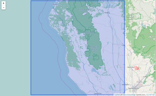
Where is the bounding box? (you’ll need lawn, or you can vizualize some other way)
library("lawn")
lawn::lawn_bbox_polygon(bbox) %>% view
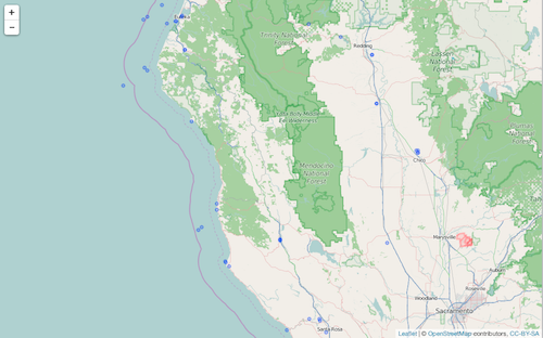
Vizualize station subset - yep, looks right
library("leaflet")
leaflet(data = out) %>%
  addTiles() %>%
  addCircles()
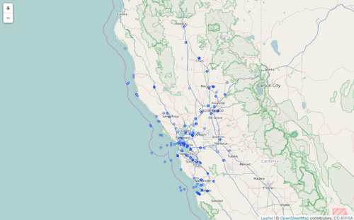
Next, search with a lat/lon coordinate, with a radius. That is, we search for stations within X km from the coordinate.
out <- isd_stations_search(lat = 38.4, lon = -123, radius = 250)
head(out)
#>     usaf  wban             station_name ctry state icao elev_m    begin
#> 1 690070 93217            FRITZSCHE AAF   US    CA KOAR   43.0 19600404
#> 2 720267 23224 AUBURN MUNICIPAL AIRPORT   US    CA KAUN  466.7 20060101
#> 3 720267 99999         AUBURN MUNICIPAL   US    CA KAUN  468.0 20040525
#> 4 720406 99999      GNOSS FIELD AIRPORT   US    CA KDVO    0.6 20071114
#> 5 720576   174       UNIVERSITY AIRPORT   US    CA KEDU   21.0 20130101
#> 6 720576 99999                    DAVIS   US    CA KEDU   21.0 20080721
#>        end      lon    lat
#> 1 19930831 -121.767 36.683
#> 2 20150831 -121.082 38.955
#> 3 20051231 -121.082 38.955
#> 4 20150831 -122.550 38.150
#> 5 20150831 -121.783 38.533
#> 6 20121231 -121.783 38.533
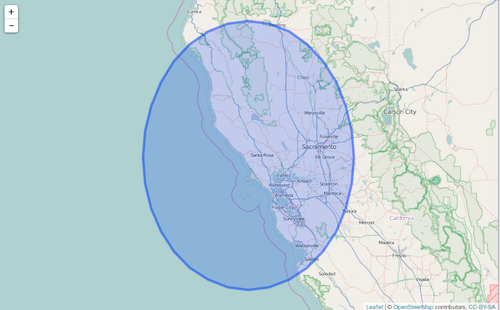
Again, compare search area to stations found
search area
pt <- lawn::lawn_point(c(-123, 38.4))
lawn::lawn_buffer(pt, dist = 250) %>% view
stations found
leaflet(data = out) %>%
  addTiles() %>%
  addCircles()
ISD data
Get ISD data
Here, I get data for four stations.
res1 <- isd(usaf="011690", wban="99999", year=1993)
res2 <- isd(usaf="172007", wban="99999", year=2015)
res3 <- isd(usaf="702700", wban="00489", year=2015)
res4 <- isd(usaf="109711", wban=99999, year=1970)
Then, combine data, with rnoaa:::rbind.isd()
res_all <- rbind(res1, res2, res3, res4)
Add date time
library("lubridate")
res_all$date_time <- ymd_hm(
  sprintf("%s %s", as.character(res_all$date), res_all$time)
)
Remove 999’s (NOAA’s way to indicate missing/no data)
library("dplyr")
res_all <- res_all %>% filter(temperature < 900)
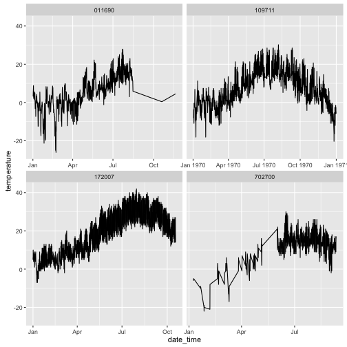
Visualize ISD data
library("ggplot2")
ggplot(res_all, aes(date_time, temperature)) +
  geom_line() +
  facet_wrap(~usaf_station, scales = "free_x")