Reply All is a great podcast. I’ve been wanting to learn some text analysis tools, and transcripts from the podcast are on their site.
Took some approaches outlined in the tidytext package in this vignette, and used the tokenizers package, and some of the tidyverse.
Code on github at sckott/nonoyes
Also check out the html version
Setup
Load deps
library("httr")
library("xml2")
library("stringi")
library("dplyr")
library("ggplot2")
library("tokenizers")
library("tidytext")
library("tidyr")
source helper functions
source("funs.R")
set base url
ra_base <- "https://gimletmedia.com/show/reply-all/episodes"
URLs
Make all urls for each page of episodes
urls <- c(ra_base, file.path(ra_base, "page", 2:8))
Get urls for each episode
res <- lapply(urls, get_urls)
Remove those that are rebroadcasts, updates, or revisited
res <- grep("rebroadcast|update|revisited", unlist(res), value = TRUE, invert = TRUE)
Episode names
Give some episodes numbers that don’t have them
epnames <- sub("/$", "", sub("https://gimletmedia.com/episode/", "", res))
epnames <- sub("the-anxiety-box", "8-the-anxiety-box", epnames)
epnames <- sub("french-connection", "10-french-connection", epnames)
epnames <- sub("ive-killed-people-and-i-have-hostages", "15-ive-killed-people-and-i-have-hostages", epnames)
epnames <- sub("6-this-proves-everything", "75-this-proves-everything", epnames)
epnames <- sub("zardulu", "56-zardulu", epnames)
Transcripts
Get transcripts
txts <- lapply(res, transcript_fetch, sleep = 1)
Parse transcripts
txtsp <- lapply(txts, transcript_parse)
Summary word usage
Summarise data for each transcript
dat <- stats::setNames(lapply(txtsp, function(m) {
  bind_rows(lapply(m, function(v) {
    tmp <- unname(vapply(v, nchar, 1))
    data_frame(
      n = length(tmp),
      mean = mean(tmp),
      n_laugh = count_word(v, "laugh"),
      n_groan = count_word(v, "groan")
    )
  }), .id = "name")
}), epnames)
Bind data together to single dataframe, and filter, summarise
data <- bind_rows(dat, .id = "episode") %>%
  filter(!is.na(episode)) %>%
  filter(grepl("^PJ$|^ALEX GOLDMAN$", name)) %>%
  mutate(ep_no = as.numeric(strextract(episode, "^[0-9]+"))) %>%
  group_by(ep_no) %>%
  mutate(nrow = NROW(ep_no)) %>%
  ungroup() %>%
  filter(nrow == 2)
data
#> # A tibble: 114 × 8
#>                 episode         name     n      mean n_laugh n_groan ep_no
#>                   <chr>        <chr> <int>     <dbl>   <int>   <int> <dbl>
#> 1            73-sandbox           PJ    89 130.65169       9       0    73
#> 2            73-sandbox ALEX GOLDMAN    25  44.00000       1       1    73
#> 3       72-dead-is-paul           PJ   137  67.77372      17       0    72
#> 4       72-dead-is-paul ALEX GOLDMAN    90  61.82222       8       0    72
#> 5  71-the-picture-taker           PJ    74  77.70270       3       0    71
#> 6  71-the-picture-taker ALEX GOLDMAN    93 105.94624       6       0    71
#> 7        69-disappeared           PJ    72  76.50000       2       0    69
#> 8        69-disappeared ALEX GOLDMAN    50 135.90000       5       0    69
#> 9      68-vampire-rules           PJ   142  88.00704       6       0    68
#> 10     68-vampire-rules ALEX GOLDMAN   117  73.16239      13       0    68
#> # ... with 104 more rows, and 1 more variables: nrow <int>
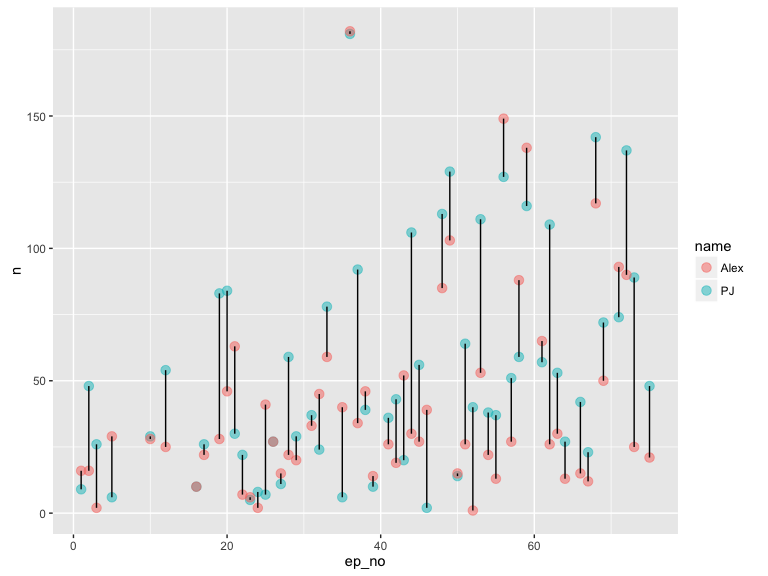
Number of words - seems PJ talks more, but didn’t do quantiative comparison
ggplot(data, aes(ep_no, n, colour = name)) +
  geom_point(size = 3, alpha = 0.5) +
  geom_line(aes(group = ep_no), colour = "black") +
  scale_color_discrete(labels = c('Alex', 'PJ'))
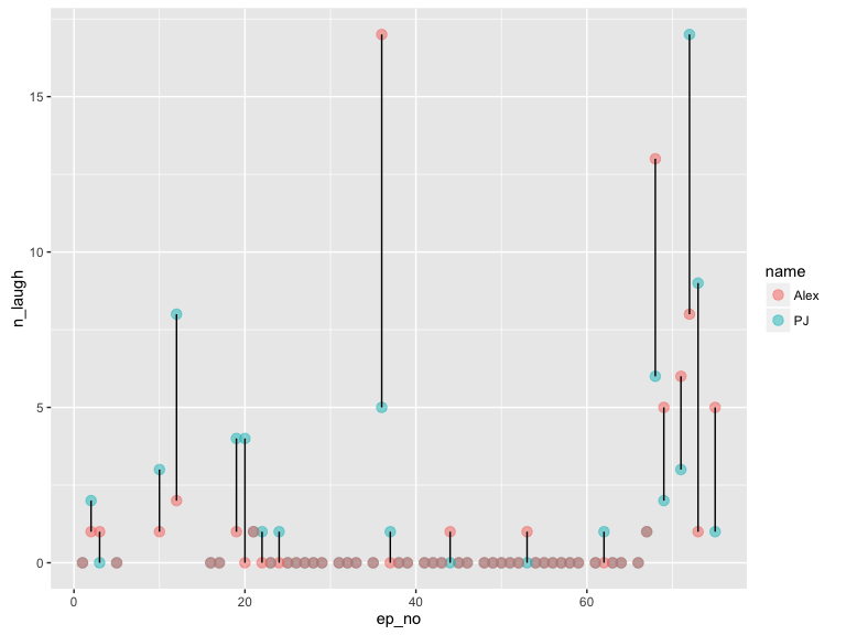
Laughs per episode - take home: PJ laughs a lot
ggplot(data, aes(ep_no, n_laugh, colour = name)) +
  geom_point(size = 3, alpha = 0.5) +
  geom_line(aes(group = ep_no), colour = "black") +
  scale_color_discrete(labels = c('Alex', 'PJ'))
Sentiment
zero <- which(vapply(txtsp, length, 1) == 0)
txtsp_ <- Filter(function(x) length(x) != 0, txtsp)
Tokenize words, and create data_frame
wordz <- stats::setNames(
  lapply(txtsp_, function(z) {
    bind_rows(
      if (is.null(try_tokenize(z$`ALEX GOLDMAN`))) {
        data_frame()
      } else {
        data_frame(
          name = "Alex",
          word = try_tokenize(z$`ALEX GOLDMAN`)
        )
      },
      if (is.null(try_tokenize(z$PJ))) {
        data_frame()
      } else {
        data_frame(
          name = "PJ",
          word = try_tokenize(z$PJ)
        )
      }
    )
  }), epnames[-zero])
Combine to single data_frame
(wordz_df <- bind_rows(wordz, .id = "episode"))
#> # A tibble: 104,713 × 3
#>       episode  name      word
#>         <chr> <chr>     <chr>
#> 1  73-sandbox  Alex      alex
#> 2  73-sandbox  Alex   goldman
#> 3  73-sandbox  Alex         i
#> 4  73-sandbox  Alex generally
#> 5  73-sandbox  Alex     don’t
#> 6  73-sandbox  Alex      alex
#> 7  73-sandbox  Alex    really
#> 8  73-sandbox  Alex      alex
#> 9  73-sandbox  Alex    groans
#> 10 73-sandbox  Alex        so
#> # ... with 104,703 more rows
Calculate sentiment using tidytext
bing <- sentiments %>%
  filter(lexicon == "bing") %>%
  select(-score)
sent <- wordz_df %>%
  inner_join(bing) %>%
  count(name, episode, sentiment) %>%
  spread(sentiment, n, fill = 0) %>%
  mutate(sentiment = positive - negative) %>%
  ungroup() %>%
  filter(!is.na(episode)) %>%
  complete(episode, name) %>%
  mutate(ep_no = as.numeric(strextract(episode, "^[0-9]+")))
sent
#> # A tibble: 148 × 6
#>                                        episode  name negative positive
#>                                          <chr> <chr>    <dbl>    <dbl>
#> 1  1-an-app-sends-a-stranger-to-say-i-love-you  Alex       19       30
#> 2  1-an-app-sends-a-stranger-to-say-i-love-you    PJ       14       14
#> 3                         10-french-connection  Alex       15       32
#> 4                         10-french-connection    PJ       16       36
#> 5     11-did-errol-morris-brother-invent-email  Alex       NA       NA
#> 6     11-did-errol-morris-brother-invent-email    PJ       25       30
#> 7                           12-backend-trouble  Alex       20       15
#> 8                           12-backend-trouble    PJ       40       59
#> 9                              13-love-is-lies  Alex       NA       NA
#> 10                             13-love-is-lies    PJ       45       64
#> # ... with 138 more rows, and 2 more variables: sentiment <dbl>,
#> #   ep_no <dbl>
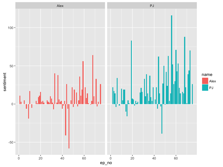
Names separate
ggplot(sent, aes(ep_no, sentiment, fill = name)) +
  geom_bar(stat = "identity") +
  facet_wrap(~name, ncol = 2, scales = "free_x")
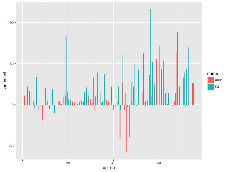
Compare for each episode
ggplot(sent, aes(ep_no, sentiment, fill = name)) +
  geom_bar(stat = "identity", position = position_dodge(width = 0.5), width = 0.6)
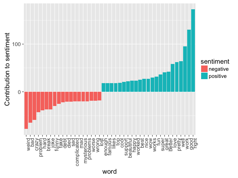
Most common positive and negative words
Clearly, the word like is surely rarely used as a positive word
meaning e.g., that they like something, but rather as the colloquial
like, totally usage. So it’s removed.
Alex
sent_cont_plot(wordz_df, "Alex")
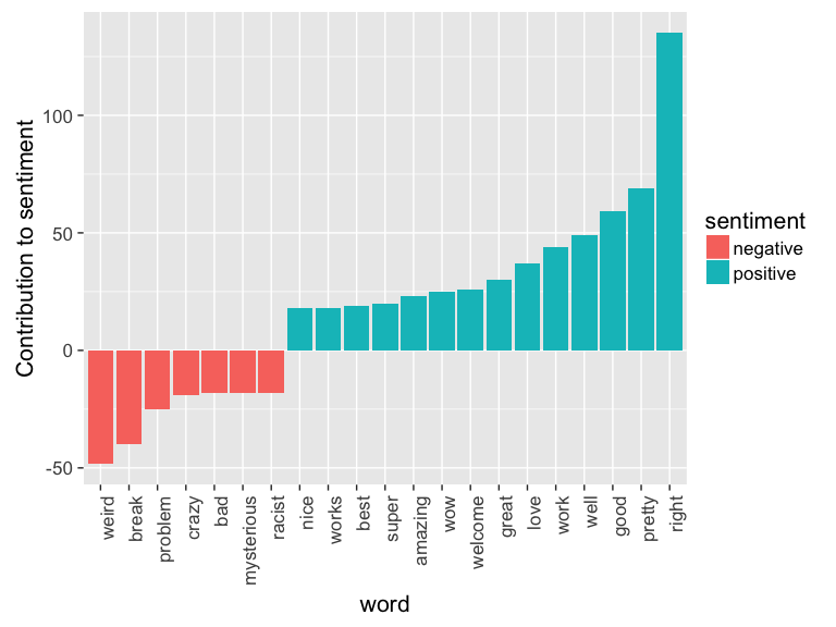
PJ
sent_cont_plot(wordz_df, "PJ")
