Why Butte County?
I went to college at California State University, Chico - in Butte County, CA. I did a BA degree in Biology there. It was a great program as it was heavily focused on natural history - with classes on herps, birds, insects, fish, etc.
Specimen collections data
Specimen collections data are increasingly being digitized, and often accessed via largeish platforms like GBIF and iDigBio. Here I’ll explore Butte County data found with iDigBio with the spocc R package. You could also use the ridigbio package to go directly to iDigBio data.
Get some data
Get county GeoJSON data using jqr
library(jqr)
butte <- jq(url("https://eric.clst.org/assets/wiki/uploads/Stuff/gz_2010_us_050_00_5m.json"), '.features[] | select(.properties.NAME == "Butte" and .properties.STATE == "06")')
mean_lon <- mean(as.numeric(jq(butte, ".geometry.coordinates[][] | first")))
mean_lat <- mean(as.numeric(jq(butte, ".geometry.coordinates[][] | last")))
Install spocc
if (!requireNamespace("spocc")) install.packages("spocc")
library(spocc)
Search for data in Butte County. First lets get a look at how many records there are:
opts <- list(rq = list(
  stateprovince = "California",
  county = "Butte",
  geopoint = list(type = "exists")
))
res <- occ(from = "idigbio", idigbioopts = opts, limit = 1)
res$idigbio$meta$found
#> [1] 45075
Looks like 45075 records found. Now let’s get all those records
res <- occ(from = "idigbio", idigbioopts = opts, limit = 46000L)
Make a map!
res$idigbio$data$custom_query$name <- res$idigbio$data$custom_query$name[1]
library(mapr)
mapr::map_leaflet(res) %>%
  leaflet::addGeoJSON(butte) %>%
  leaflet::setView(mean_lon, mean_lat, 10)
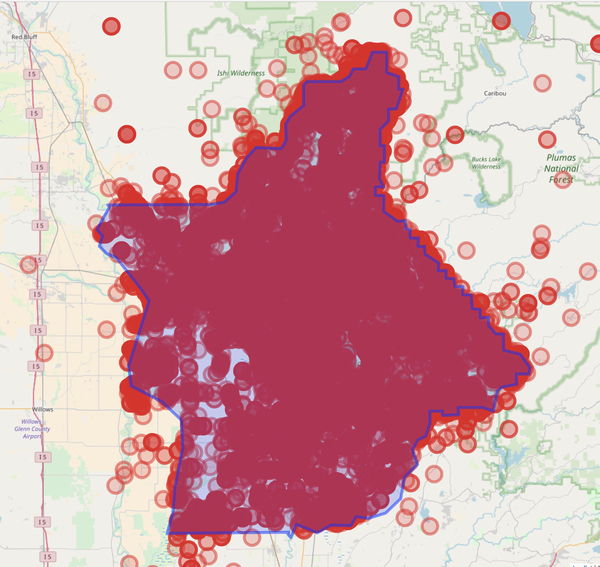
note: there’s definitely points that fall outside of Butte County, but we’ll ignore those for simplicity sake
What’s the taxonomic breakdown like?
library(dplyr)
df <- res$idigbio$data$custom_query
(x <- df %>%
    group_by(class) %>%
    summarise(n = n()) %>%
    arrange(desc(n)))
#> # A tibble: 42 x 2
#>    class              n
#>    <chr>          <int>
#>  1 magnoliopsida  25449
#>  2 liliopsida      9174
#>  3 <NA>            6355
#>  4 insecta         1490
#>  5 polypodiopsida   891
#>  6 pinopsida        351
#>  7 aves             283
#>  8 bryopsida        255
#>  9 lycopodiopsida   161
#> 10 equisetopsida     99
#> # ... with 32 more rows
Looks like the vast, vast majority are plants, and more specifically Magnoliopsida (56%). About 3% are insects; about 0.6% birds; 0.1% reptiles; and 0.11% mammals.
First, get Butte County data in a sp class
library(sp)
library(ggplot2)

county <- map_data("county")
butte_co <- filter(county, region == "california", subregion == "butte")
butte_poly <- SpatialPolygons(list(Polygons(list(Polygon(butte_co[, c(1,2)])), ID=1)))
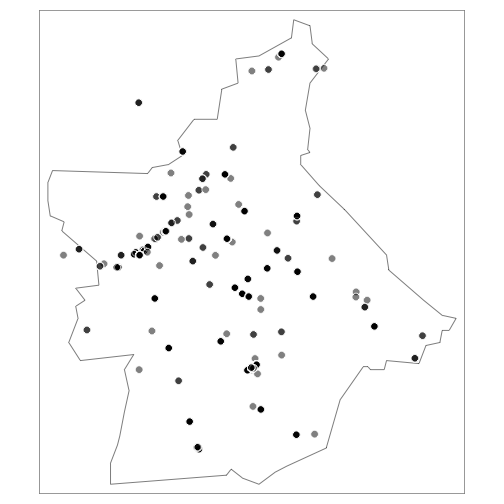
Insects:
library(tmap)
insects <- df %>% dplyr::filter(class == "insecta")
coordinates(insects) <- c('longitude', 'latitude')
tm_shape(butte_poly) +
  tm_borders() +
  tm_shape(insects) +
  tm_symbols(col = "black", border.col = "white", size = 0.5, alpha = 0.5)
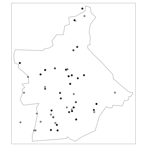
Birds:
birds <- df %>% dplyr::filter(class == "aves")
coordinates(birds) <- c('longitude', 'latitude')
tm_shape(butte_poly) +
  tm_borders() +
  tm_shape(birds) +
  tm_symbols(col = "black", border.col = "white", size = 0.5, alpha = 0.5)
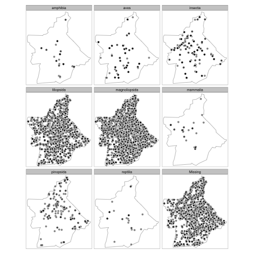
Facet by taxonomic group
library(sp)
library(rgeos)
library(ggplot2)
library(tmap)

# get subset of data for particular classes
# this is a very large portion of the data
df_class_subset <- df %>% filter(class %in% c("magnoliopsida", "liliopsida", NA,
  "insecta", "pinopsida", "aves", "amphibia", "mammalia", "reptilia"))
coordinates(df_class_subset) <- c('longitude', 'latitude')

# get butte county data into a polygon
county <- map_data("county")
butte_co <- filter(county, region == "california", subregion == "butte")
butte_poly <- SpatialPolygons(list(Polygons(list(Polygon(butte_co[, c(1,2)])), ID=1)))

# clip data to butte county
df_class_subset_clipped <- raster::intersect(df_class_subset, butte_poly)

tm_shape(butte_poly) +
  tm_borders() +
  tm_shape(df_class_subset_clipped) +
  tm_symbols(col = "black", border.col = "white", size = 0.5, alpha = 0.5) +
  tm_facets(by = "class", nrow = 3, free.coords = FALSE)
Collectors. Lowell Ahart is kind of a legend in Butte County, collecting plants like crazy. Let’s see how many records he has
df %>% filter(grepl("ahart", collector, ignore.case = TRUE))
#> # A tibble: 15,864 x 83
#>    associatedsequenc… barcodevalue basisofrecord   bed   canonicalname
#>    <lgl>              <lgl>        <chr>           <lgl> <chr>
#>  1 NA                 NA           preservedspeci… NA    isolepis setacea
#>  2 NA                 NA           preservedspeci… NA    fallopia convolv…
#>  3 NA                 NA           preservedspeci… NA    carex densa
#>  4 NA                 NA           preservedspeci… NA    datura wrightii
#>  5 NA                 NA           preservedspeci… NA    hieracium argutum
#>  6 NA                 NA           preservedspeci… NA    centunculus mini…
#>  7 NA                 NA           preservedspeci… NA    dryopteris arguta
#>  8 NA                 NA           preservedspeci… NA    epilobium cleist…
#>  9 NA                 NA           preservedspeci… NA    psilocarphus ten…
#> 10 NA                 NA           preservedspeci… NA    lycium barbarum
#> # ... with 15,854 more rows, and 78 more variables: catalognumber <chr>,
#> #   class <chr>, collectioncode <chr>, collectionid <chr>,
#> #   collectionname <lgl>, collector <chr>, commonname <chr>,
#> #   commonnames <list>, continent <chr>, coordinateuncertainty <dbl>,
#> #   country <chr>, countrycode <chr>, county <chr>, datasetid <chr>,
#> #   datecollected <date>, datemodified <chr>, dqs <dbl>,
#> #   earliestageorloweststage <lgl>, earliesteonorlowesteonothem <lgl>,
#> #   earliestepochorlowestseries <chr>, earliesteraorlowesterathem <lgl>,
#> #   earliestperiodorlowestsystem <chr>, etag <chr>, eventdate <chr>,
#> #   family <chr>, fieldnumber <chr>, flags <list>, formation <chr>,
#> #   genus <chr>, geologicalcontextid <lgl>, longitude <dbl>,
#> #   latitude <dbl>, group <lgl>, hasImage <lgl>, hasMedia <lgl>,
#> #   highertaxon <chr>, highestbiostratigraphiczone <lgl>,
#> #   individualcount <int>, infraspecificepithet <chr>,
#> #   institutioncode <chr>, institutionid <chr>, institutionname <lgl>,
#> #   kingdom <chr>, latestageorhigheststage <lgl>,
#> #   latesteonorhighesteonothem <lgl>, latestepochorhighestseries <lgl>,
#> #   latesteraorhighesterathem <lgl>, latestperiodorhighestsystem <lgl>,
#> #   lithostratigraphicterms <lgl>, locality <chr>,
#> #   lowestbiostratigraphiczone <lgl>, maxdepth <lgl>, maxelevation <dbl>,
#> #   mediarecords <list>, member <lgl>, mindepth <lgl>, minelevation <dbl>,
#> #   municipality <chr>, occurrenceid <chr>, order <chr>, phylum <chr>,
#> #   recordids <list>, recordnumber <chr>, recordset <chr>, name <chr>,
#> #   specificepithet <chr>, startdayofyear <int>, stateprovince <chr>,
#> #   taxonid <chr>, taxonomicstatus <chr>, taxonrank <chr>,
#> #   typestatus <chr>, uuid <chr>, verbatimeventdate <chr>,
#> #   verbatimlocality <chr>, version <lgl>, waterbody <chr>, prov <chr>
Wow. That’s a big portion of the total records in the county.